ggplot Runthrough

ggplot Runthrough
ggplot Runthrough
ggplot Runthrough
ggplot Runthrough
ggplot Runthrough
ggplot Runthrough
ggplot Runthrough
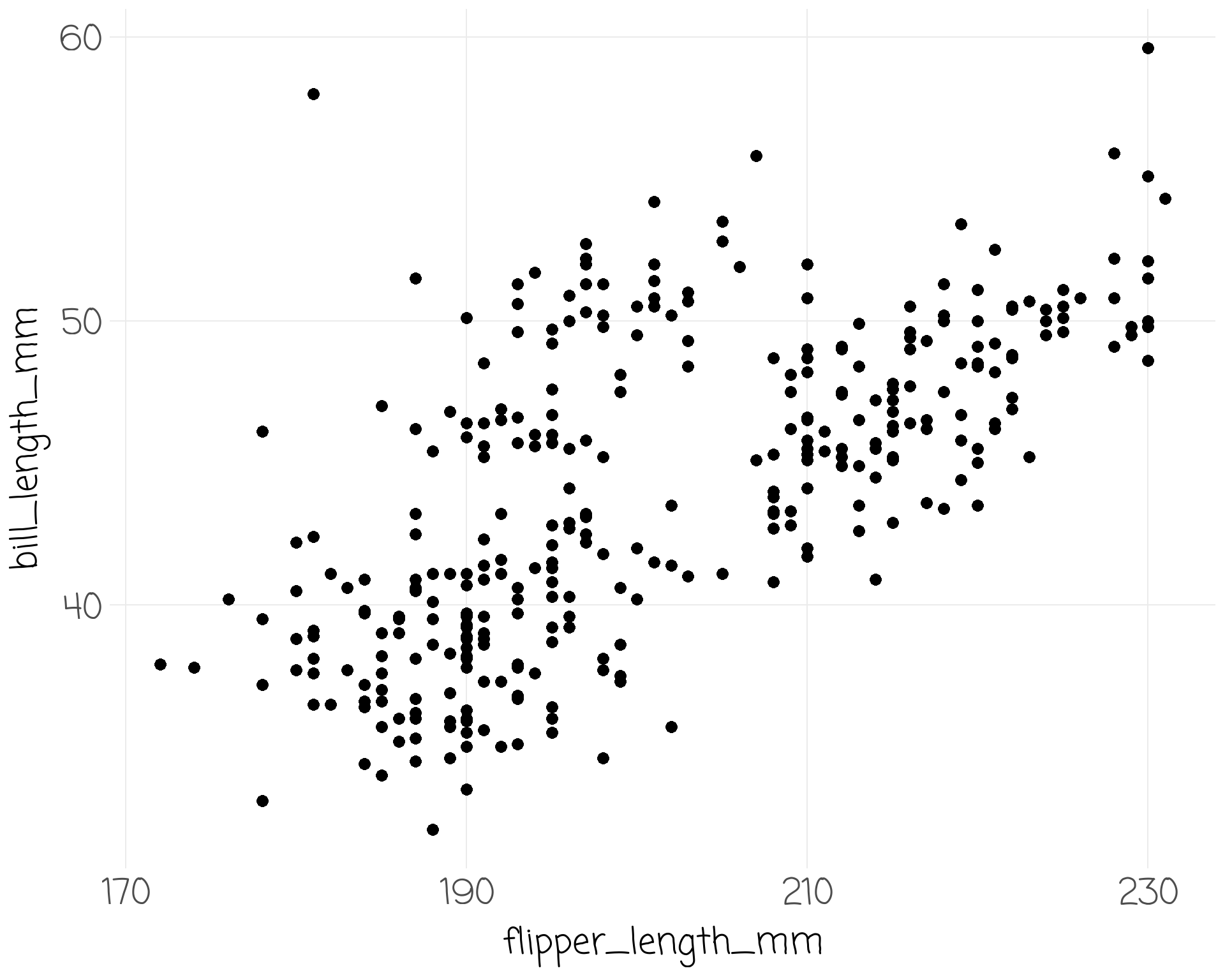
penguins %>% drop_na() %>%
ggplot() +
aes(x = flipper_length_mm) +
scale_x_continuous(breaks = seq(170, 230, by = 20)) +
aes(y = bill_length_mm) +
geom_point(size = 3, show.legend = F) +
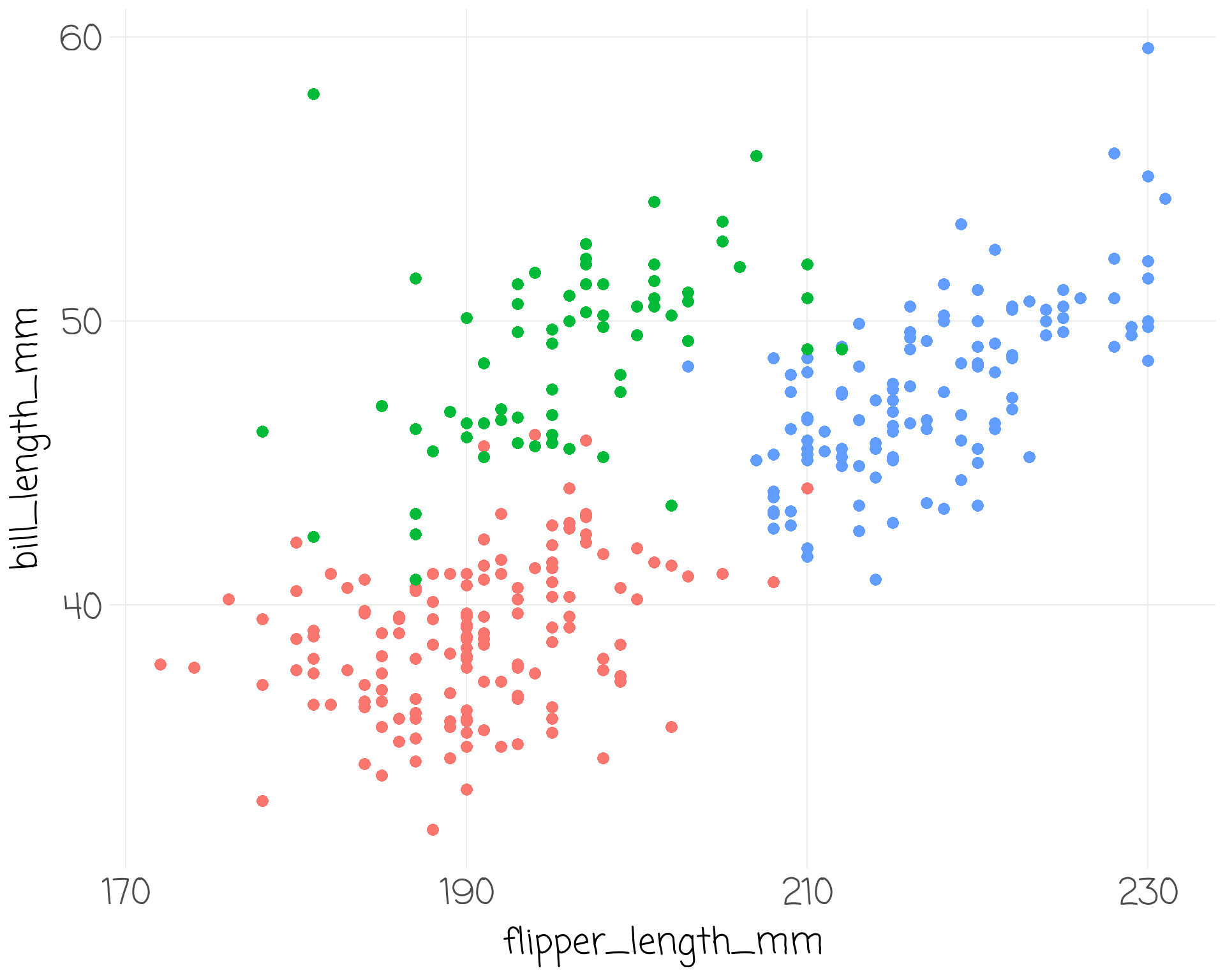
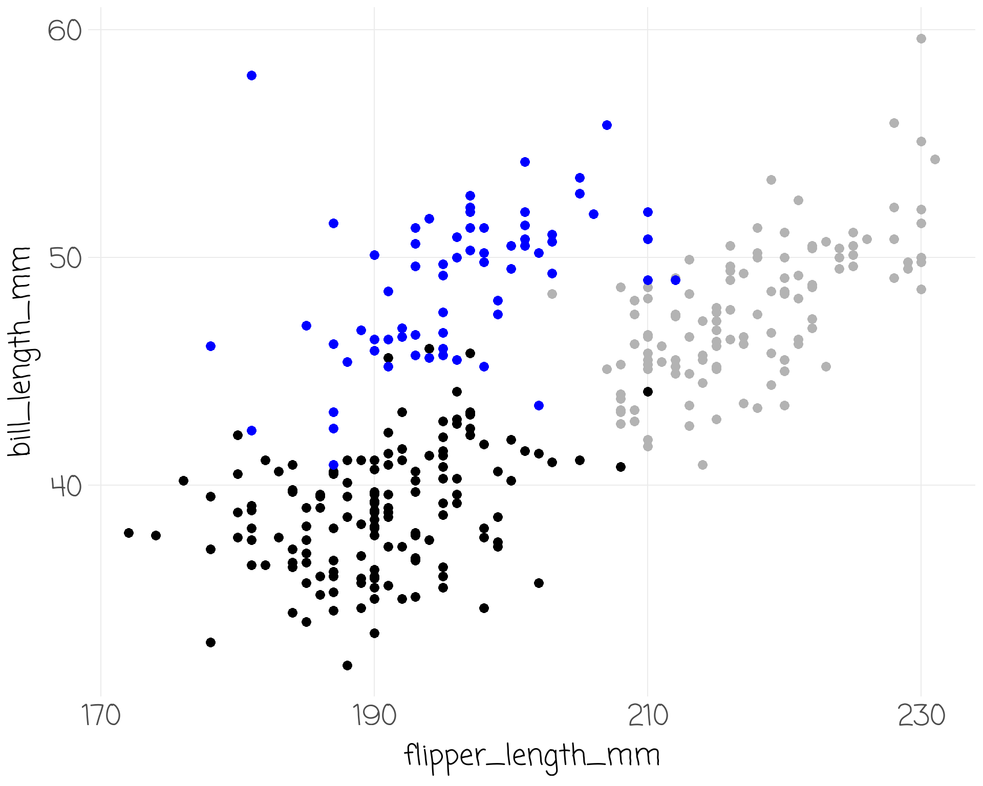
aes(colour = species) +
scale_color_manual(values = c("black", "blue", "grey70")) +
ggalt::geom_encircle(size = 5, show.legend = FALSE)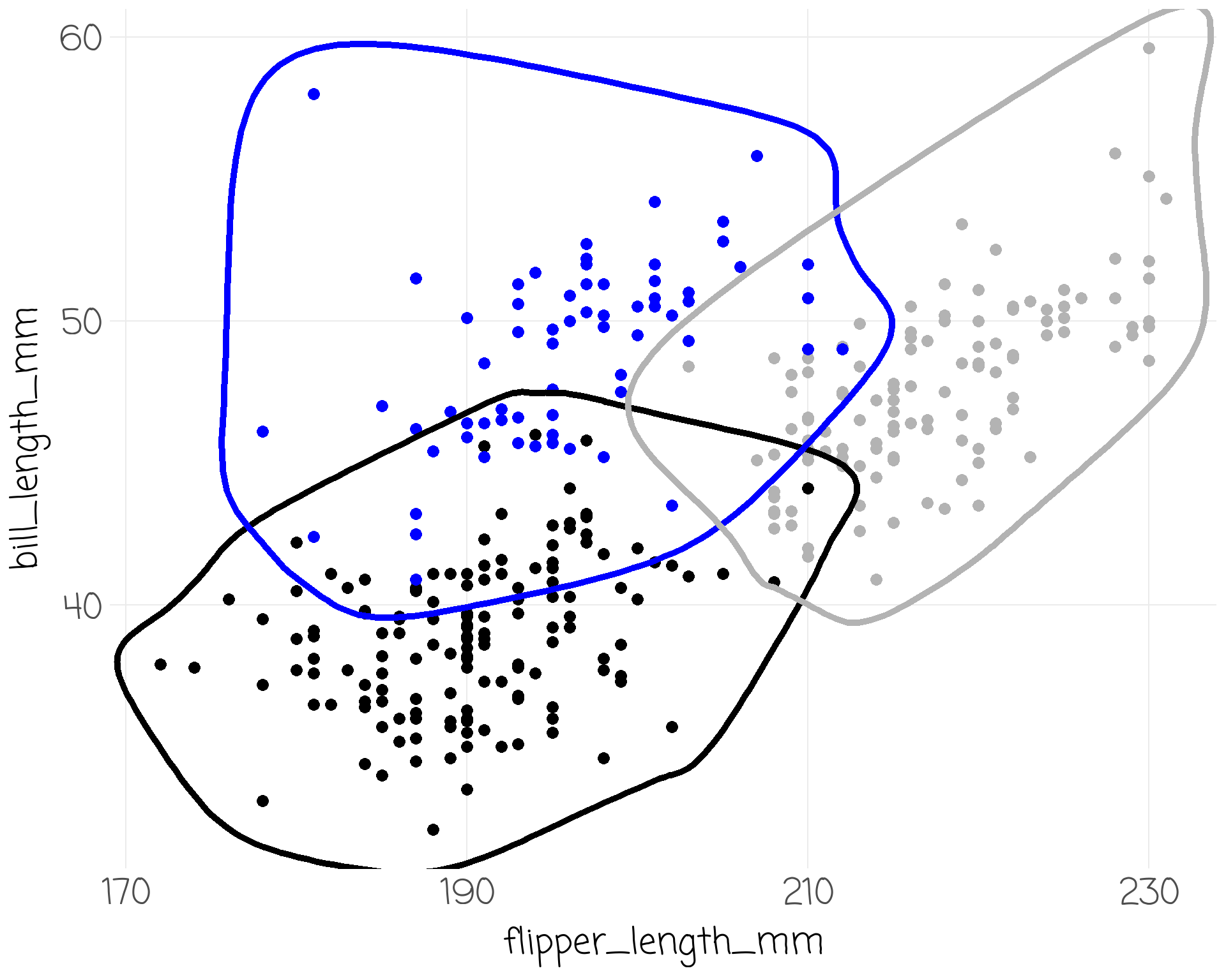
ggplot Runthrough
penguins %>% drop_na() %>%
  ggplot() +
aes(x = flipper_length_mm) +
scale_x_continuous(breaks = seq(170, 230, by = 20)) +
aes(y = bill_length_mm) +
geom_point(size = 3, show.legend = F) +
aes(colour = species) +
scale_color_manual(values = c("black", "blue", "grey70")) +
ggalt::geom_encircle(size = 5, show.legend = FALSE) +
labs(title = "Chinstraps have Short Flippers",
subtitle = "{.black Adelie}, {.blue Chinstrap}, and {.#B0B0B0 Gentoo} penguins",
x = "Flipper Length (mm)",
y = "Bill Length (mm)",
caption = "@Data from Palmer Penguins")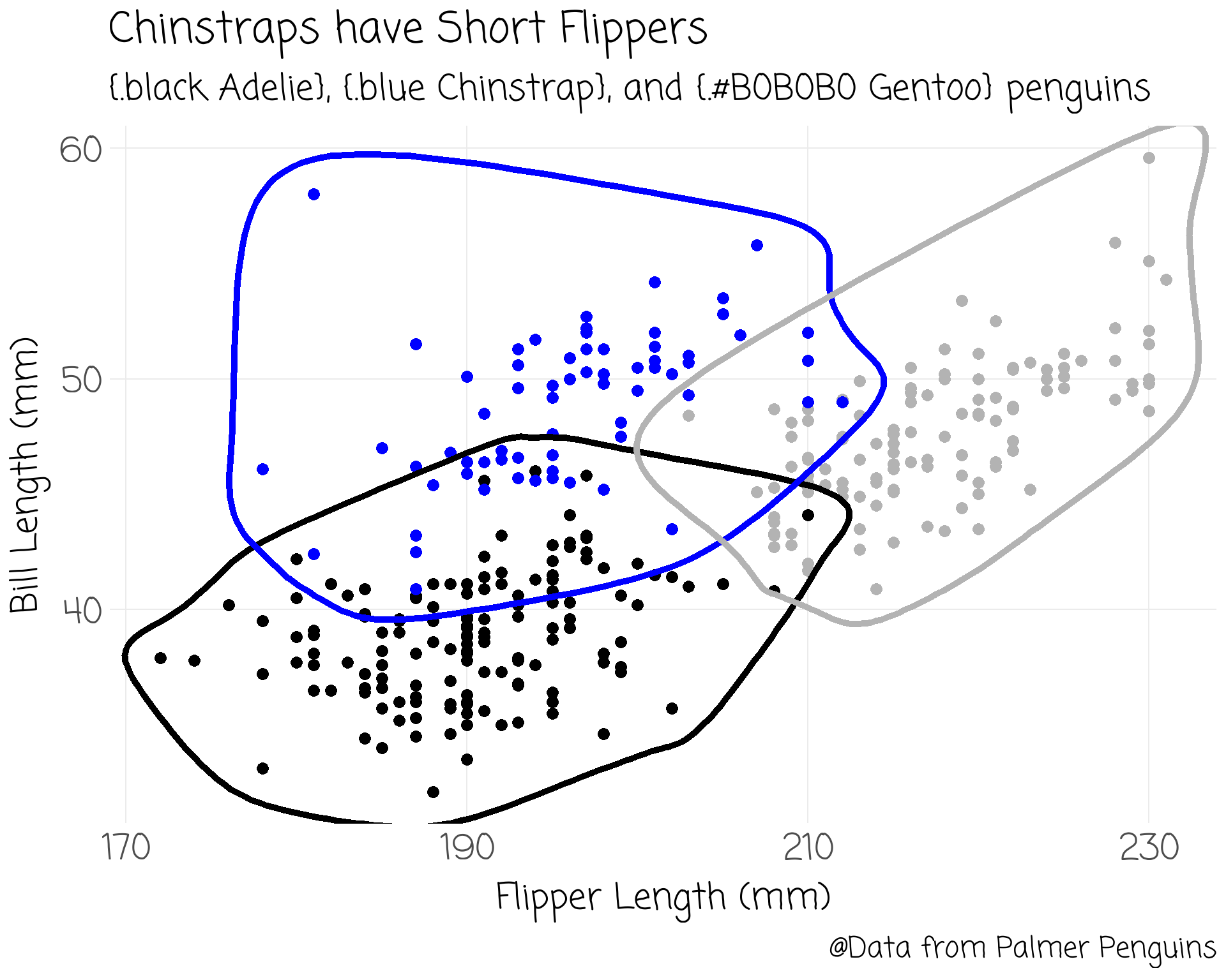
ggplot Runthrough
penguins %>% drop_na() %>%
  ggplot() +
  aes(x = flipper_length_mm) +
scale_x_continuous(breaks = seq(170, 230, by = 20)) +
aes(y = bill_length_mm) +
geom_point(size = 3, show.legend = F) +
aes(colour = species) +
scale_color_manual(values = c("black", "blue", "grey70")) +
ggalt::geom_encircle(size = 5, show.legend = FALSE) +
labs(title = "Chinstraps have Short Flippers",
subtitle = "{.black Adelie}, {.blue Chinstrap}, and {.#B0B0B0 Gentoo} penguins",
x = "Flipper Length (mm)",
y = "Bill Length (mm)",
caption = "@Data from Palmer Penguins") +
theme(text = element_text(family = "Ink Free", size = 32))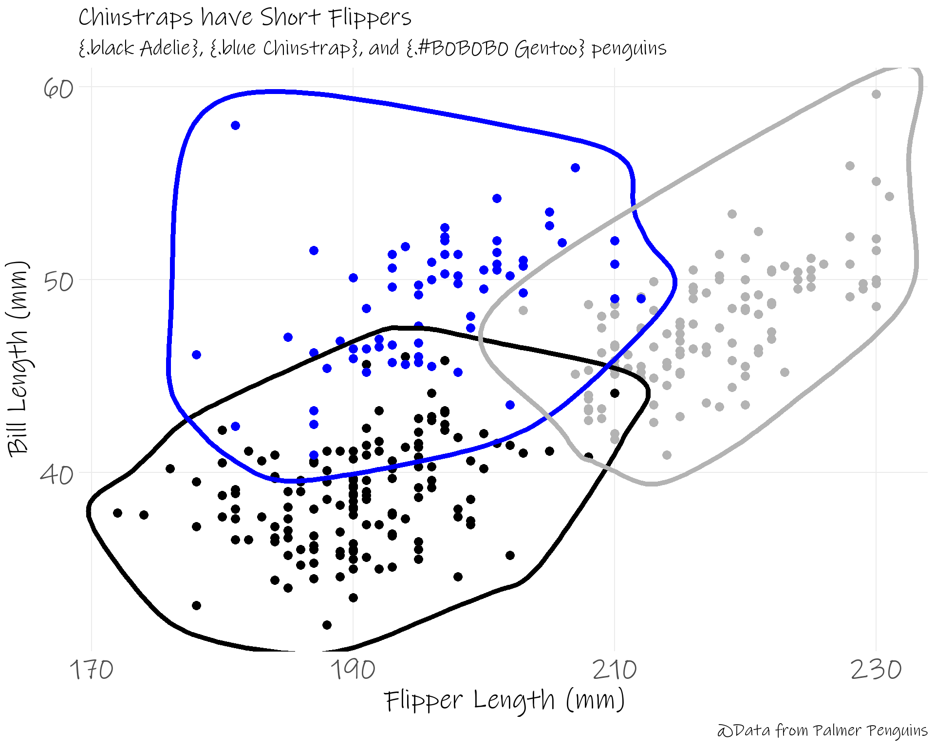
ggplot Runthrough
penguins %>% drop_na() %>%
  ggplot() +
  aes(x = flipper_length_mm) +
  scale_x_continuous(breaks = seq(170, 230, by = 20)) +
aes(y = bill_length_mm) +
geom_point(size = 3, show.legend = F) +
aes(colour = species) +
scale_color_manual(values = c("black", "blue", "grey70")) +
ggalt::geom_encircle(size = 5, show.legend = FALSE) +
labs(title = "Chinstraps have Short Flippers",
subtitle = "{.black Adelie}, {.blue Chinstrap}, and {.#B0B0B0 Gentoo} penguins",
x = "Flipper Length (mm)",
y = "Bill Length (mm)",
caption = "@Data from Palmer Penguins") +
theme(text = element_text(family = "Ink Free", size = 32)) +
theme(plot.subtitle = element_marquee(width = 1))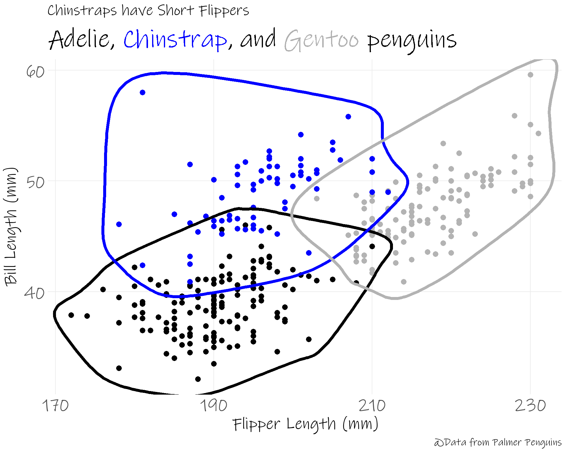
ggplot Runthrough
penguins %>% drop_na() %>%
  ggplot() +
  aes(x = flipper_length_mm) +
  scale_x_continuous(breaks = seq(170, 230, by = 20)) +
  aes(y = bill_length_mm) +
geom_point(size = 3, show.legend = F) +
aes(colour = species) +
scale_color_manual(values = c("black", "blue", "grey70")) +
ggalt::geom_encircle(size = 5, show.legend = FALSE) +
labs(title = "Chinstraps have Short Flippers",
subtitle = "{.black Adelie}, {.blue Chinstrap}, and {.#B0B0B0 Gentoo} penguins",
x = "Flipper Length (mm)",
y = "Bill Length (mm)",
caption = "@Data from Palmer Penguins") +
theme(text = element_text(family = "Ink Free", size = 32)) +
theme(plot.subtitle = element_marquee(width = 1)) +
facet_grid(~sex)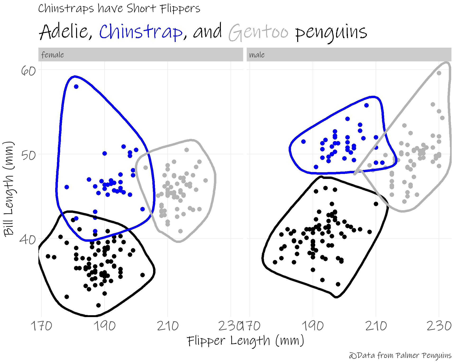
ggplot Runthrough
penguins %>% drop_na() %>%
  ggplot() +
  aes(x = flipper_length_mm) +
  scale_x_continuous(breaks = seq(170, 230, by = 20)) +
  aes(y = bill_length_mm) +
  geom_point(size = 3, show.legend = F) +
aes(colour = species) +
scale_color_manual(values = c("black", "blue", "grey70")) +
ggalt::geom_encircle(size = 5, show.legend = FALSE) +
labs(title = "Chinstraps have Short Flippers",
subtitle = "{.black Adelie}, {.blue Chinstrap}, and {.#B0B0B0 Gentoo} penguins",
x = "Flipper Length (mm)",
y = "Bill Length (mm)",
caption = "@Data from Palmer Penguins") +
theme(text = element_text(family = "Ink Free", size = 32)) +
theme(plot.subtitle = element_marquee(width = 1)) +
facet_grid(~sex)
Bar Plots
Bar Plots
Bar Plots
Bar Plots
Bar Plots
Bar Plots
Bar Plots

Bar Plots
Bar Plots

Bar Plots
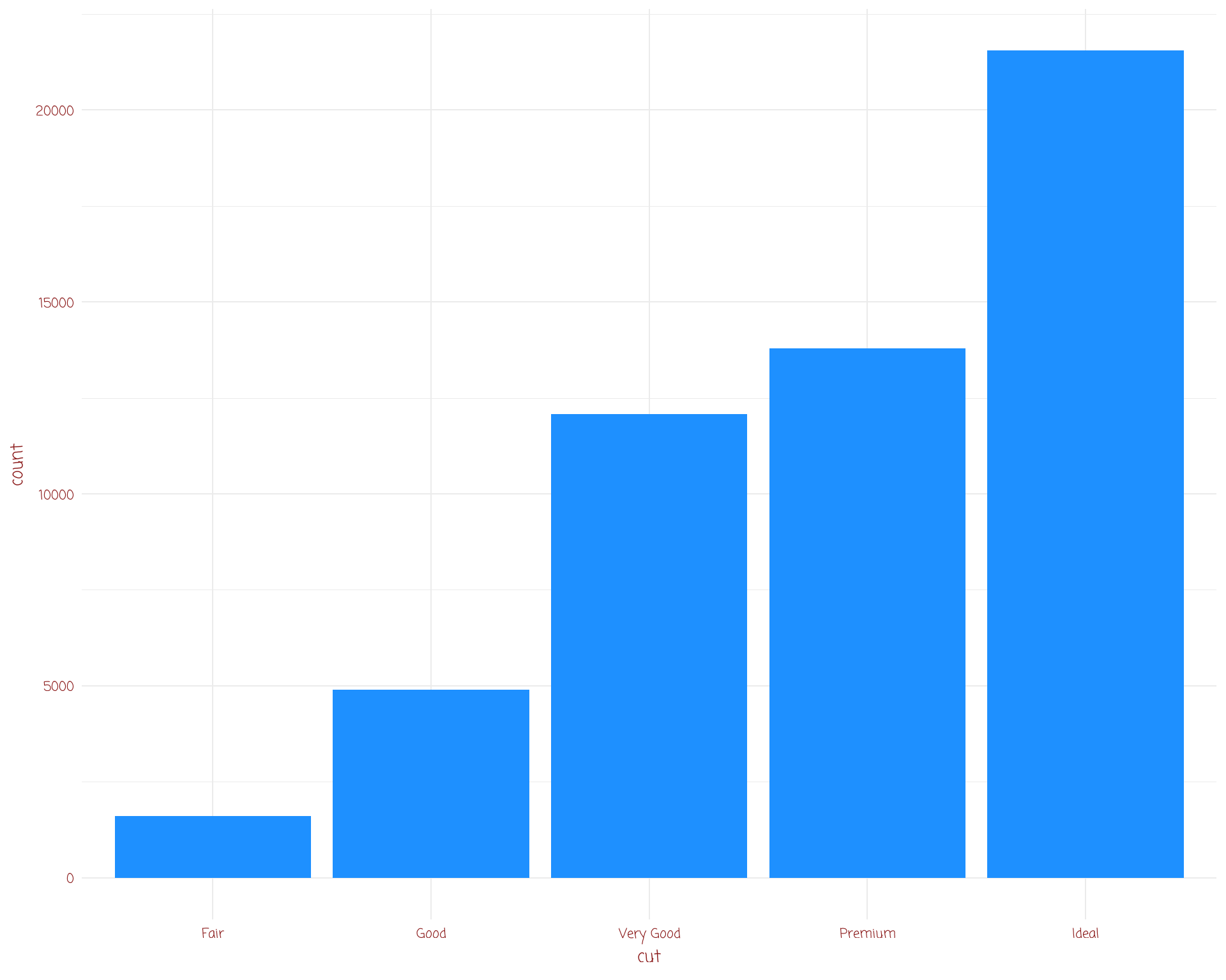
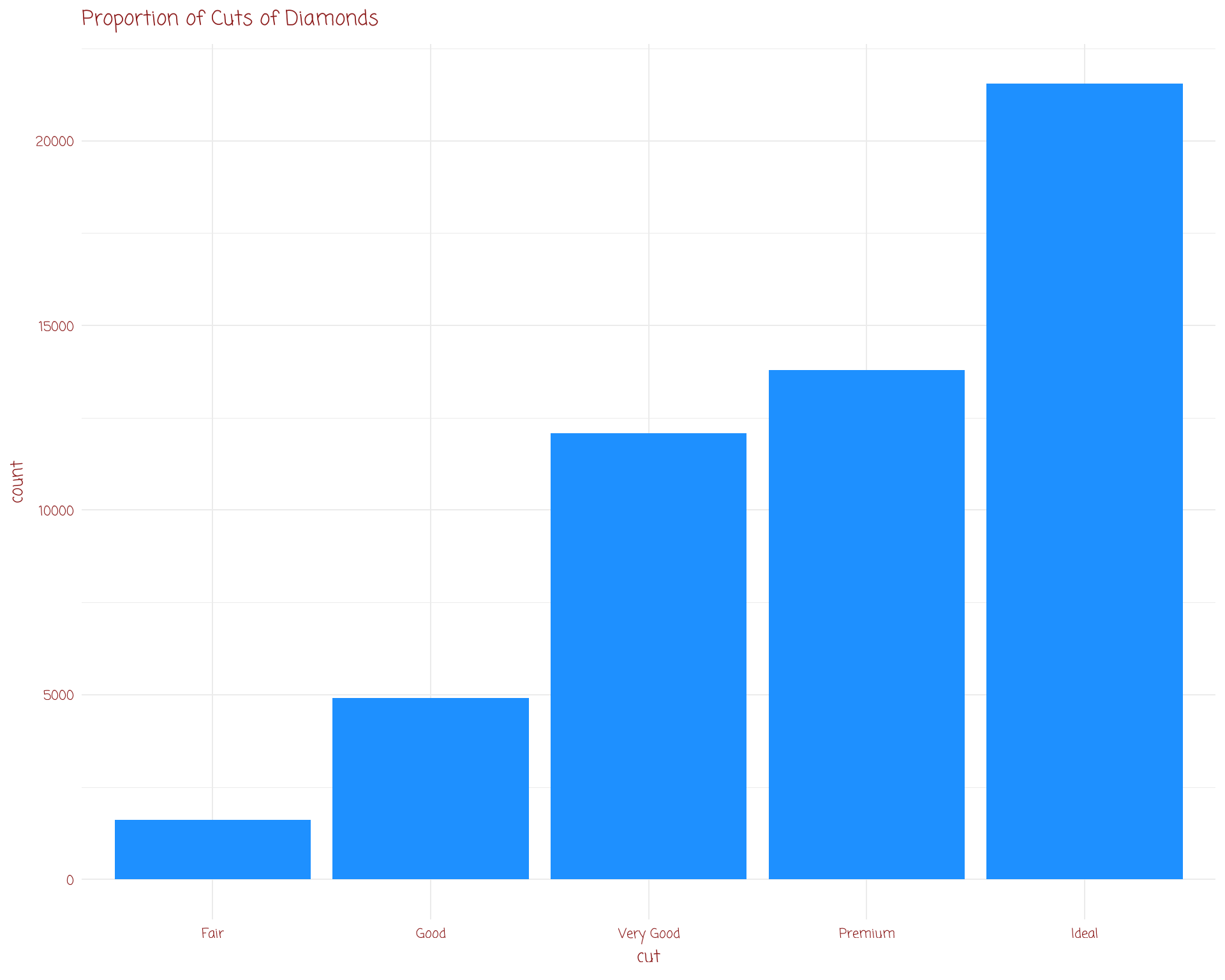
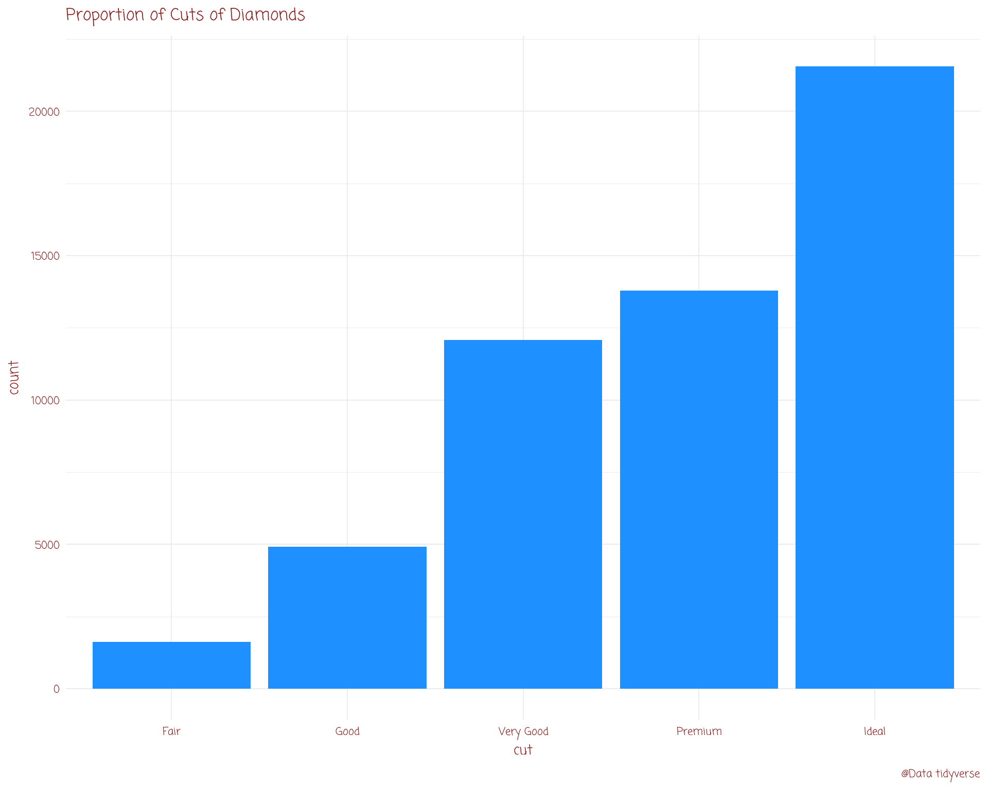
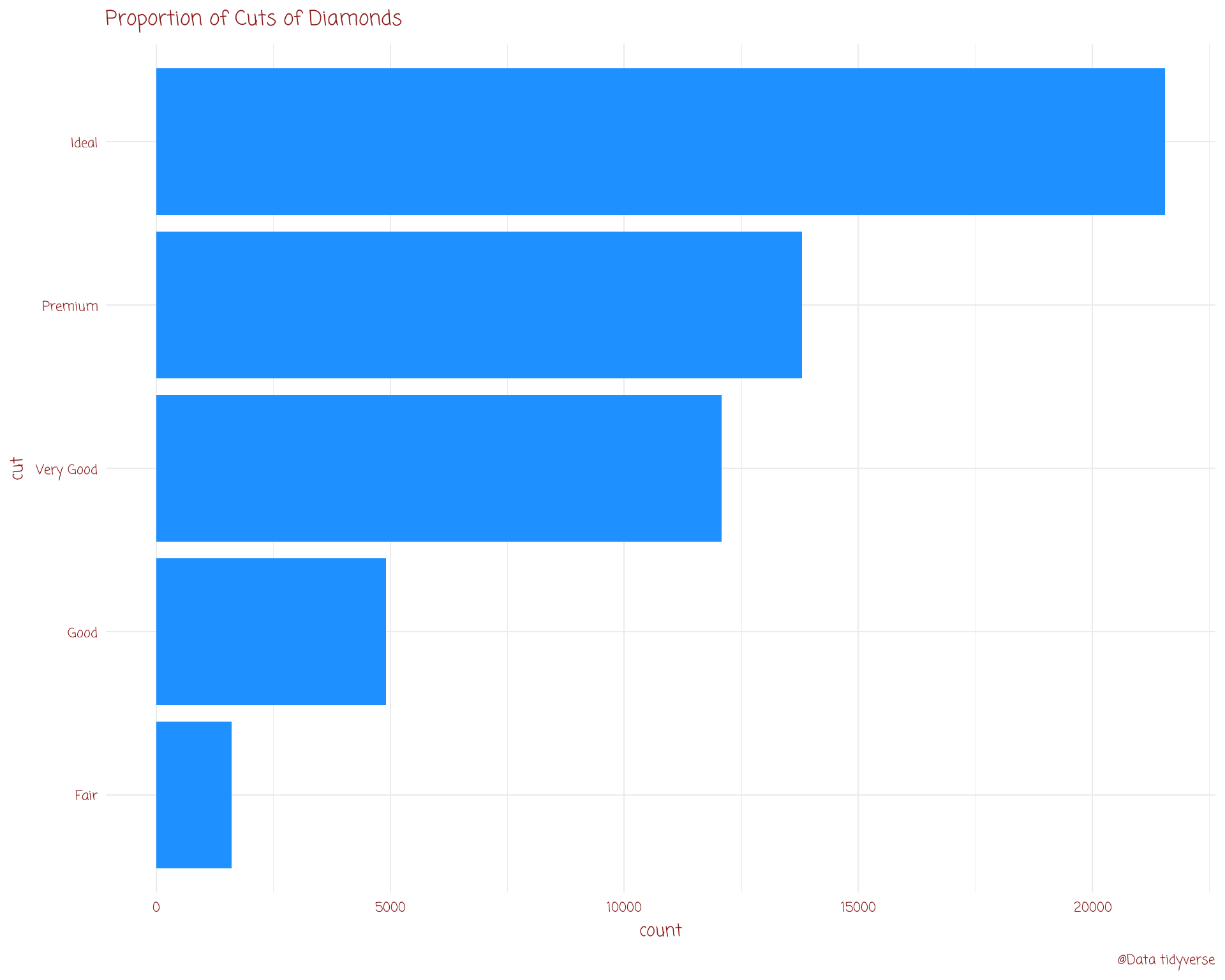
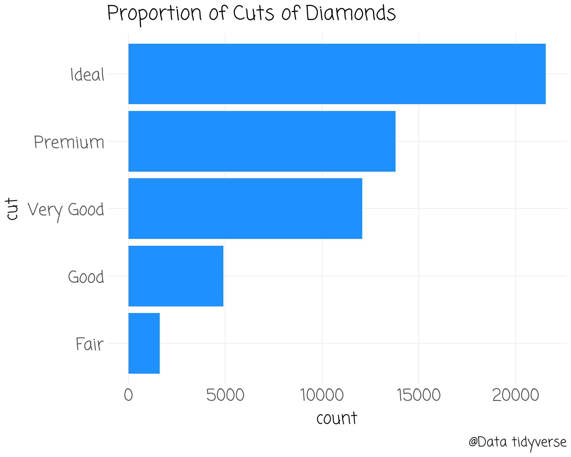
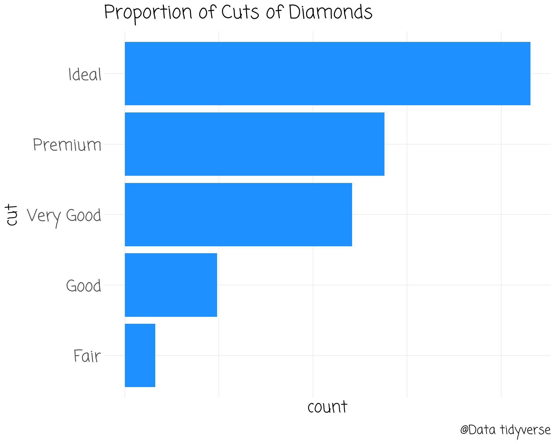
diamonds %>%
ggplot(aes(cut)) +
geom_bar(fill = "dodgerblue1") +
ggtitle("Proportion of Cuts of Diamonds") +
labs(caption = "@Data tidyverse") +
coord_flip() +
theme_clean() +
theme(text = element_text(size = 40)) +
theme(axis.text.x = element_blank()) +
theme(axis.title = element_blank()) +
theme(title = element_text(face = "bold"))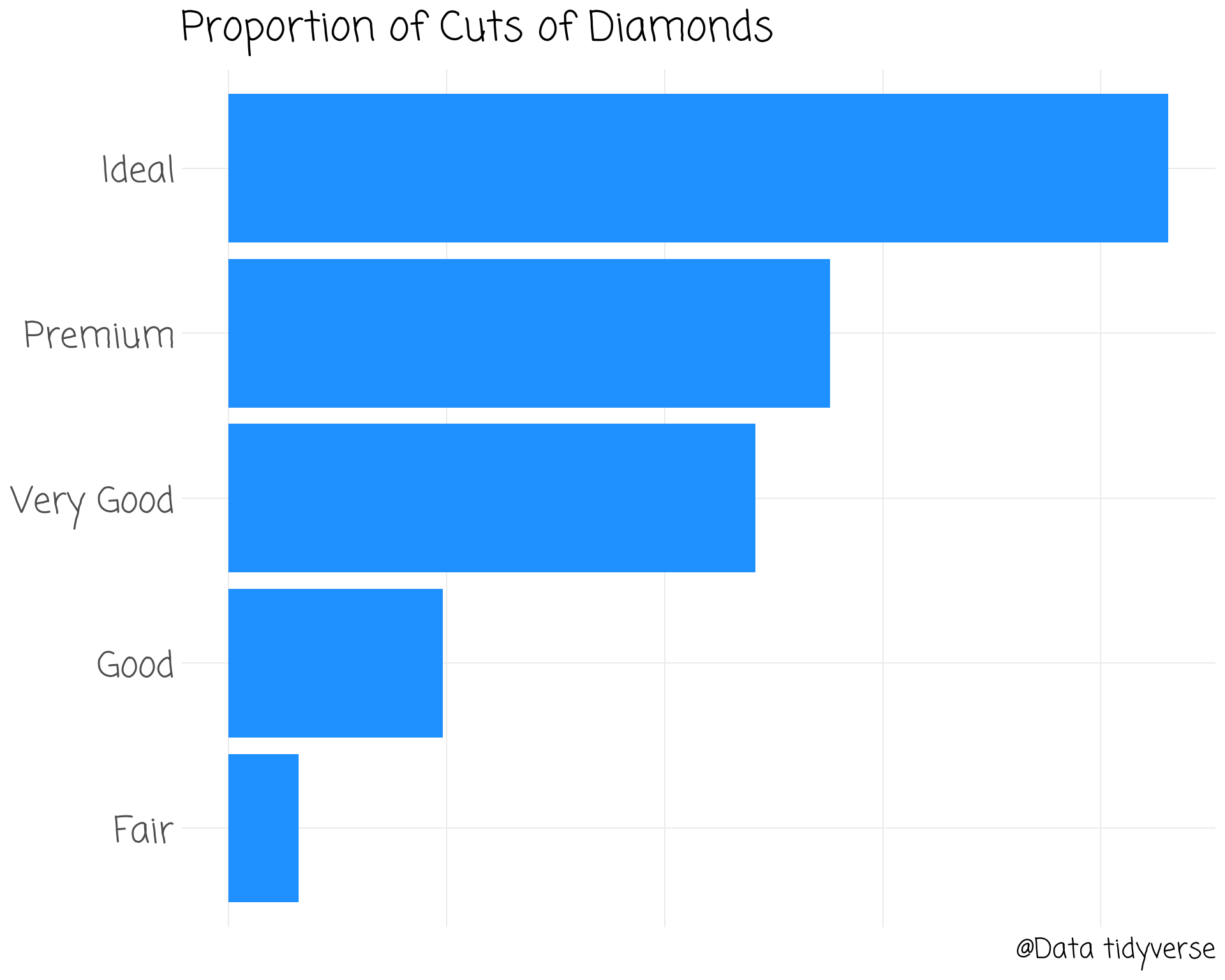
Movie Barplot
Movie Barplot
Movie Barplot
Movie Barplot
Movie Barplot
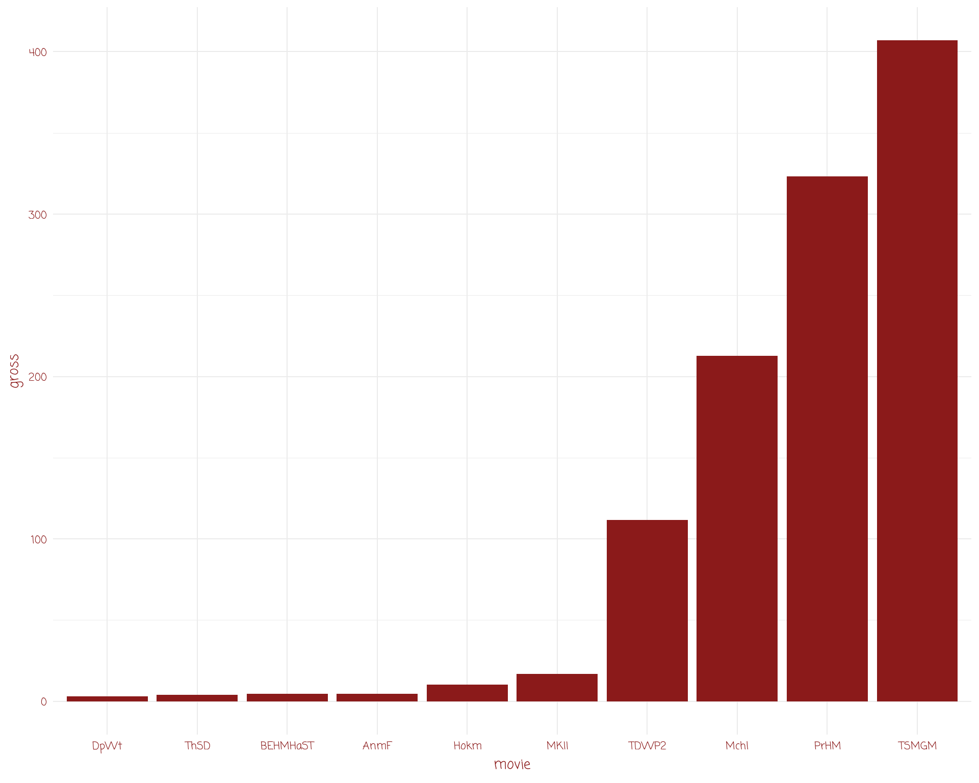
movies %>% mutate(movie = fct_reorder(movie, gross)) %>%
slice_head(n=10) %>%
ggplot(aes(movie, gross)) +
geom_col(fill = "firebrick4") +
theme_clean() +
scale_y_continuous(breaks = scales::breaks_extended(8),
labels = scales::label_dollar(scale = 1)) +
labs(title = glue::glue("Box Office {boxoffice_date_string}"),
caption = "@Data from BoxOfficeMojo",
y = "Gross (Million$)")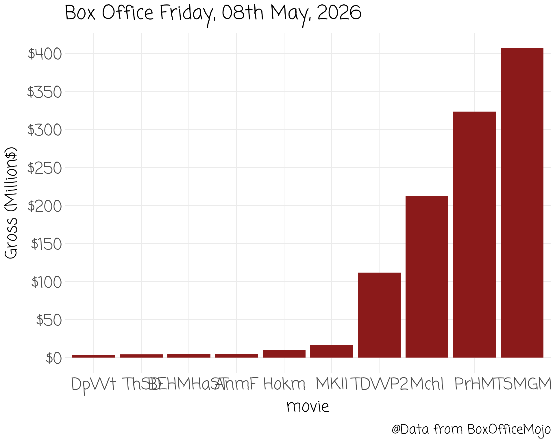
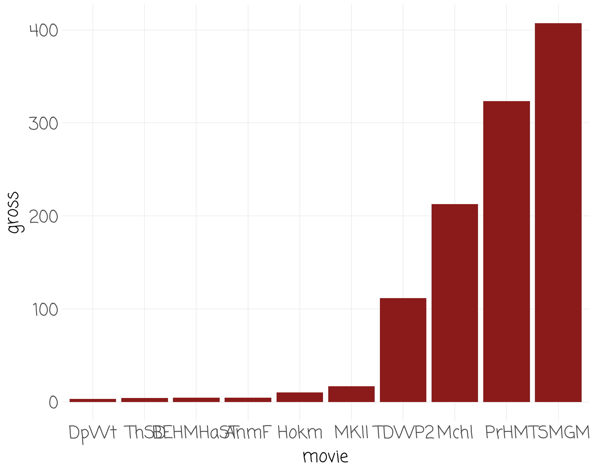
Movie Barplot
movies %>% mutate(movie = fct_reorder(movie, gross)) %>%
  slice_head(n=10) %>%
ggplot(aes(movie, gross)) +
geom_col(fill = "firebrick4") +
theme_clean() +
scale_y_continuous(breaks = scales::breaks_extended(8),
labels = scales::label_dollar(scale = 1)) +
labs(title = glue::glue("Box Office {boxoffice_date_string}"),
caption = "@Data from BoxOfficeMojo",
y = "Gross (Million$)") +
coord_flip()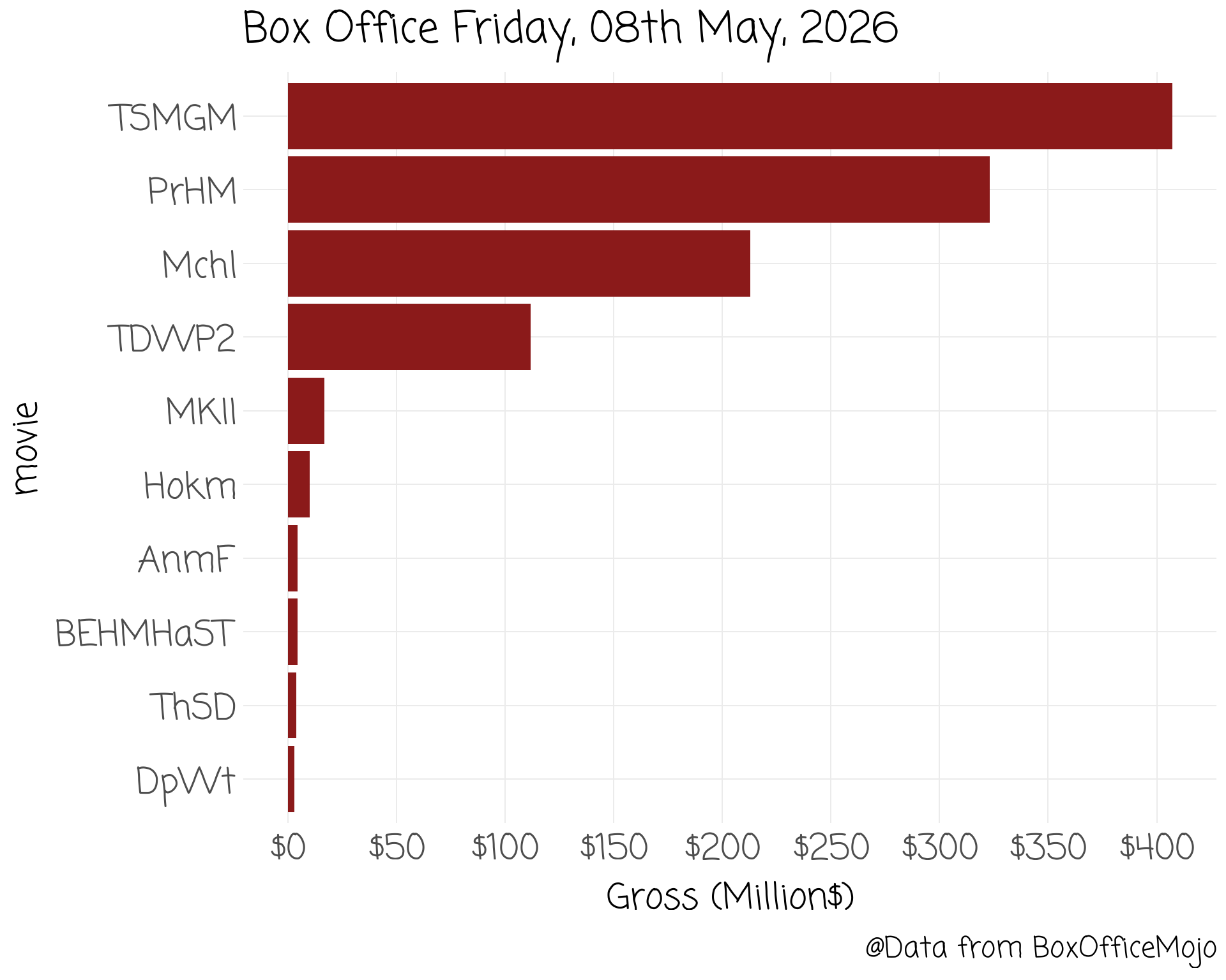
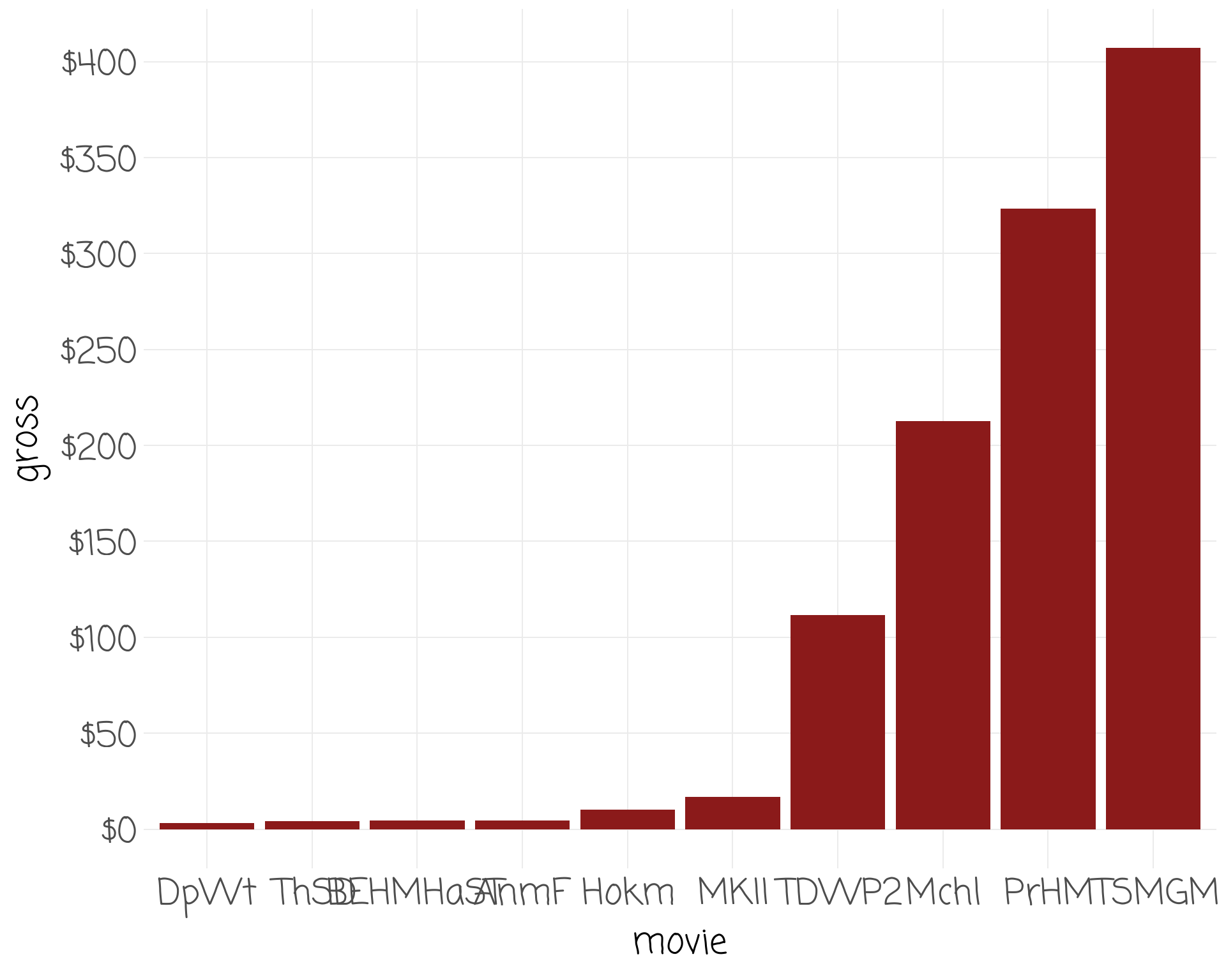
Movie Barplot
movies %>% mutate(movie = fct_reorder(movie, gross)) %>%
  slice_head(n=10) %>%
  ggplot(aes(movie, gross)) +
geom_col(fill = "firebrick4") +
theme_clean() +
scale_y_continuous(breaks = scales::breaks_extended(8),
labels = scales::label_dollar(scale = 1)) +
labs(title = glue::glue("Box Office {boxoffice_date_string}"),
caption = "@Data from BoxOfficeMojo",
y = "Gross (Million$)") +
coord_flip() +
theme(axis.title.y = element_blank())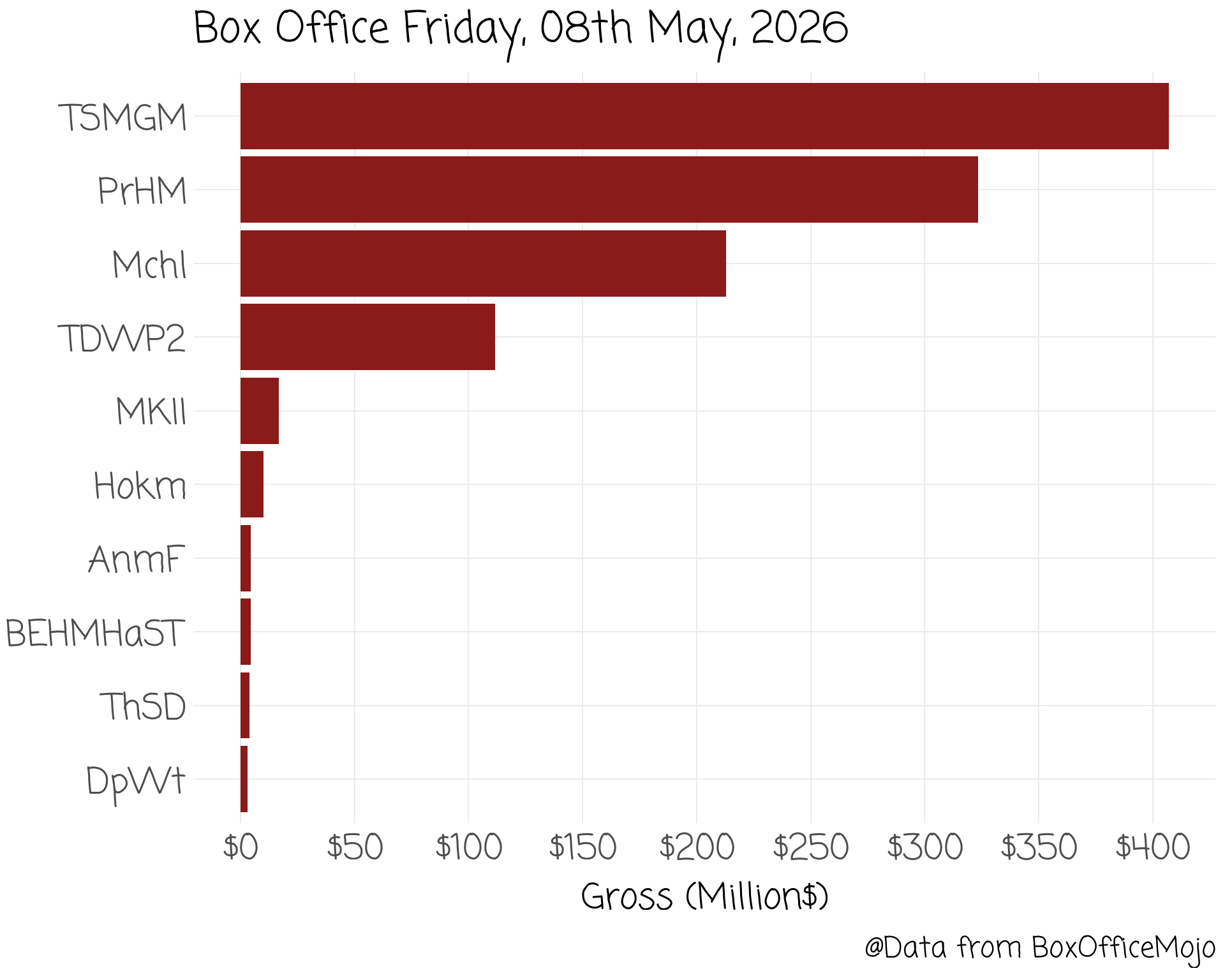
Column Plot
penguins %>%
  group_by(species) %>%
  summarise(body_mass = mean(body_mass_g, na.rm = T)) %>%
  ggplot(aes(species, body_mass, xend = species, yend = body_mass)) +
  theme_clean() +
  coord_flip() +
  labs(caption = "@PalmerPenguins",
       y = "Body Mass (g)",
       x = "") +
  ylim(c(0, 6000)) +
  geom_col(fill = "firebrick4") +
  labs(x = "")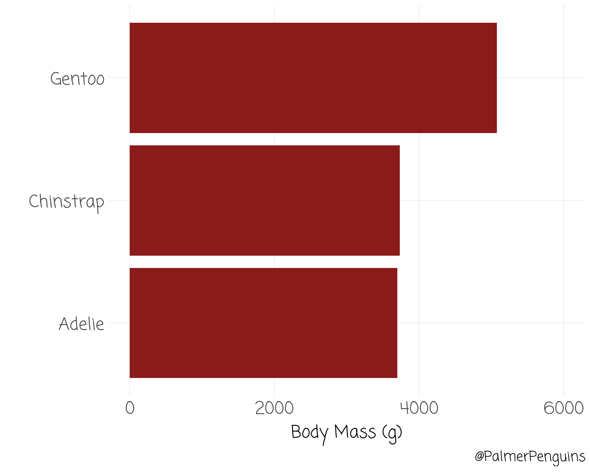
Column Plot
penguins %>%
  group_by(species) %>%
  summarise(body_mass = mean(body_mass_g, na.rm = T)) %>%
  ggplot(aes(species, body_mass, xend = species, yend = body_mass)) +
  theme_clean() +
  coord_flip() +
  labs(caption = "@PalmerPenguins",
       y = "Body Mass (g)",
       x = "") +
  ylim(c(0, 6000)) +
  geom_point(colour = "firebrick4", size = 4) +
  labs(x = "")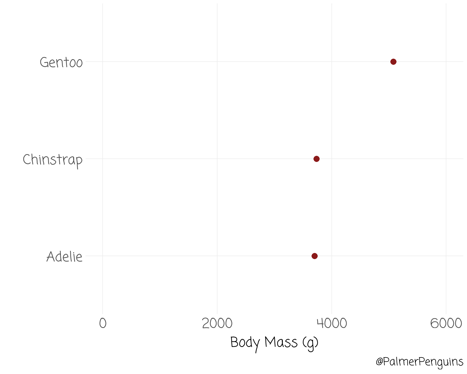
Column Plot
penguins %>%
  group_by(species) %>%
  summarise(body_mass = mean(body_mass_g, na.rm = T)) %>%
  ggplot(aes(species, body_mass, xend = species, yend = body_mass)) +
  theme_clean() +
  coord_flip() +
  labs(caption = "@PalmerPenguins",
       y = "Body Mass (g)",
       x = "") +
  ylim(c(0, 6000)) +
  geom_segment(linewidth = 2, colour = "firebrick4", y = 0) + geom_point(colour = "firebrick4", size = 4) +
  labs(x = "")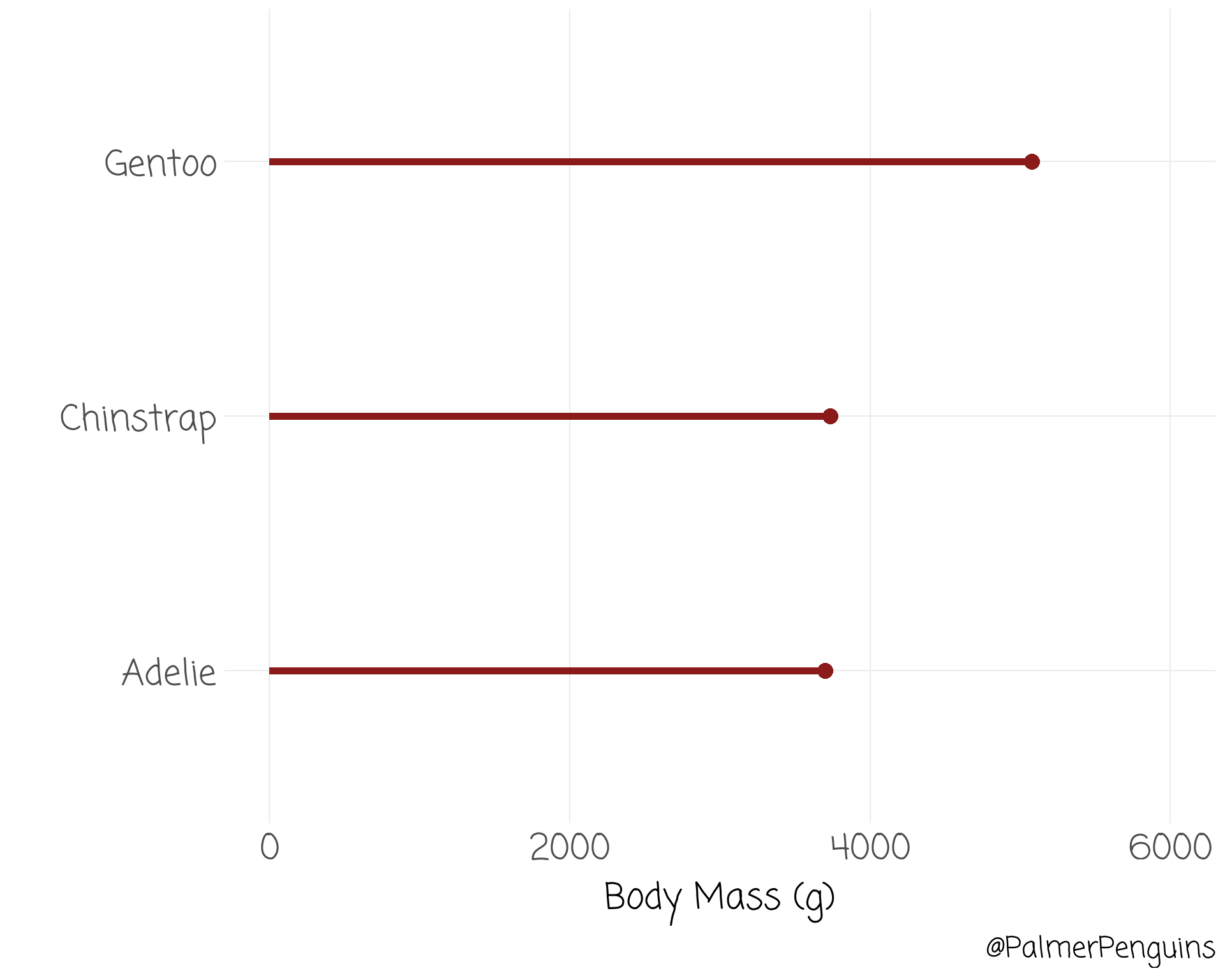
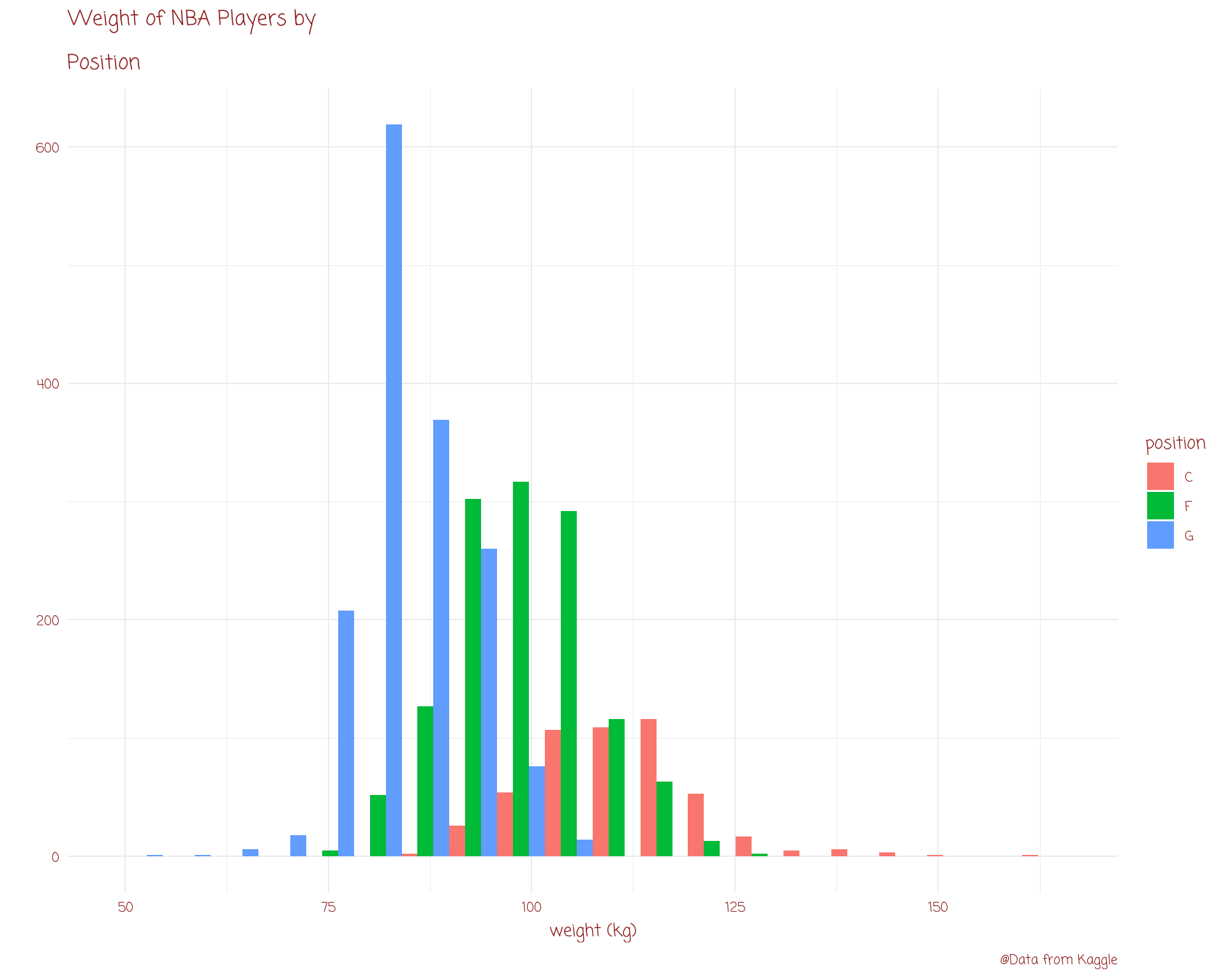
Histogram

Histogram
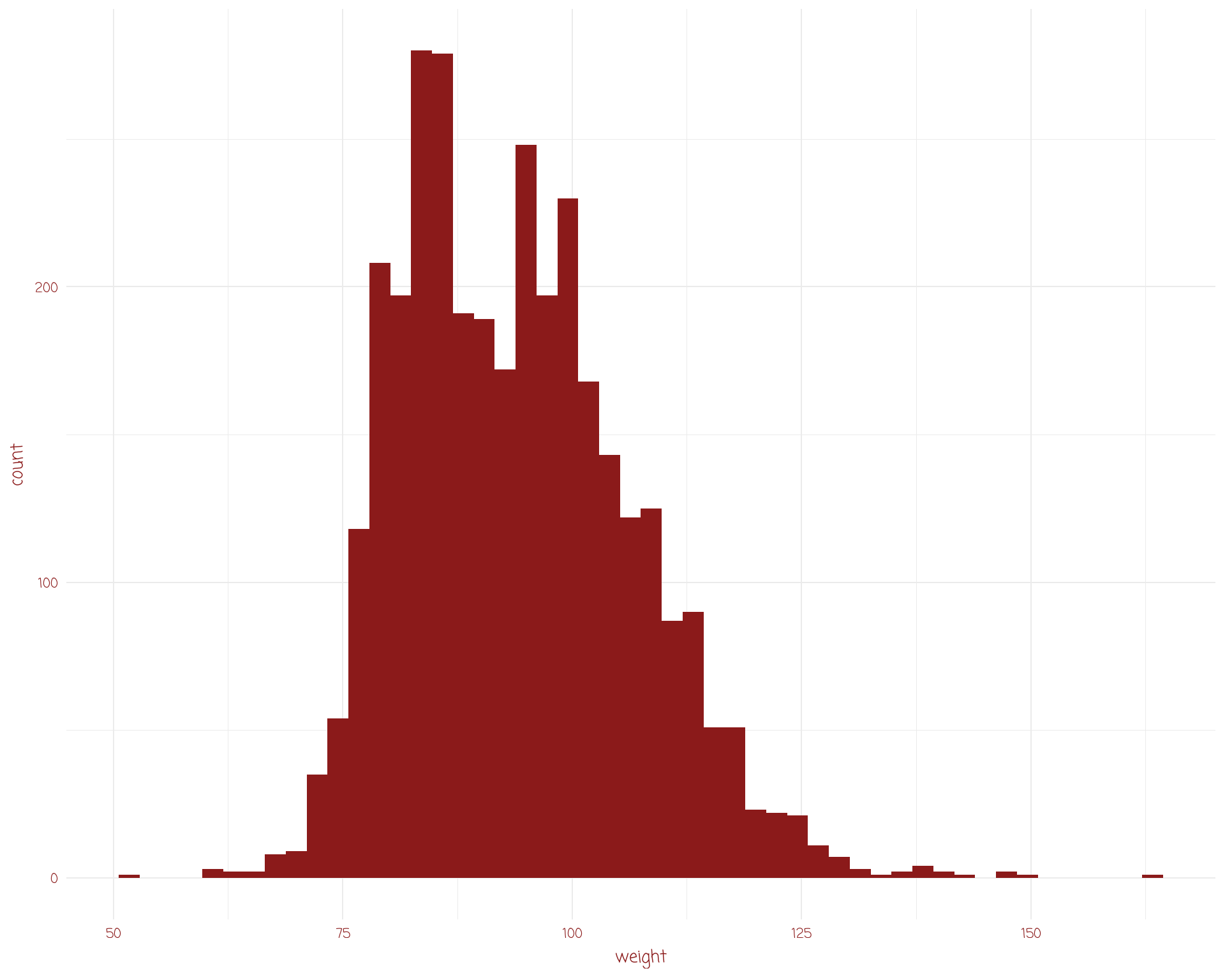
Histogram
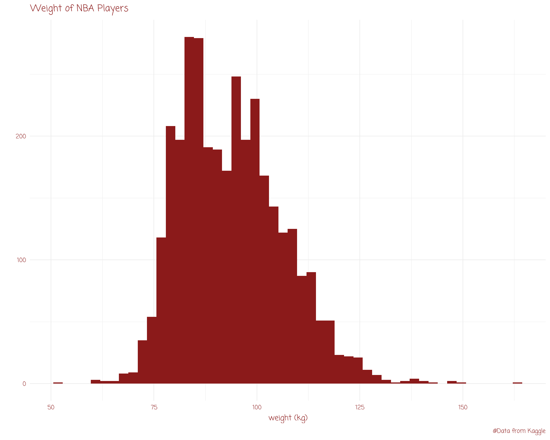
Histogram

Histogram
Histogram
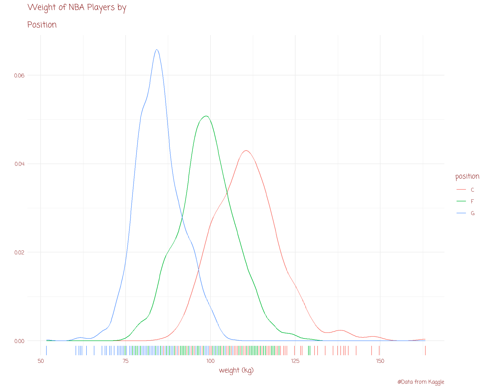
Density Plot
Density Plot
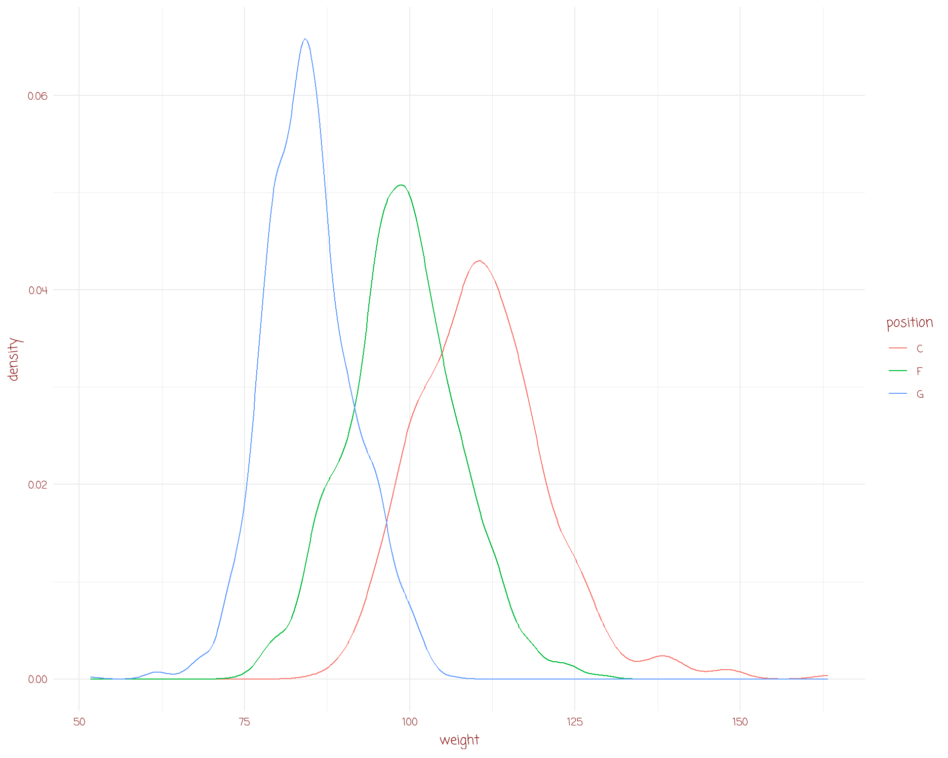
Density Plot
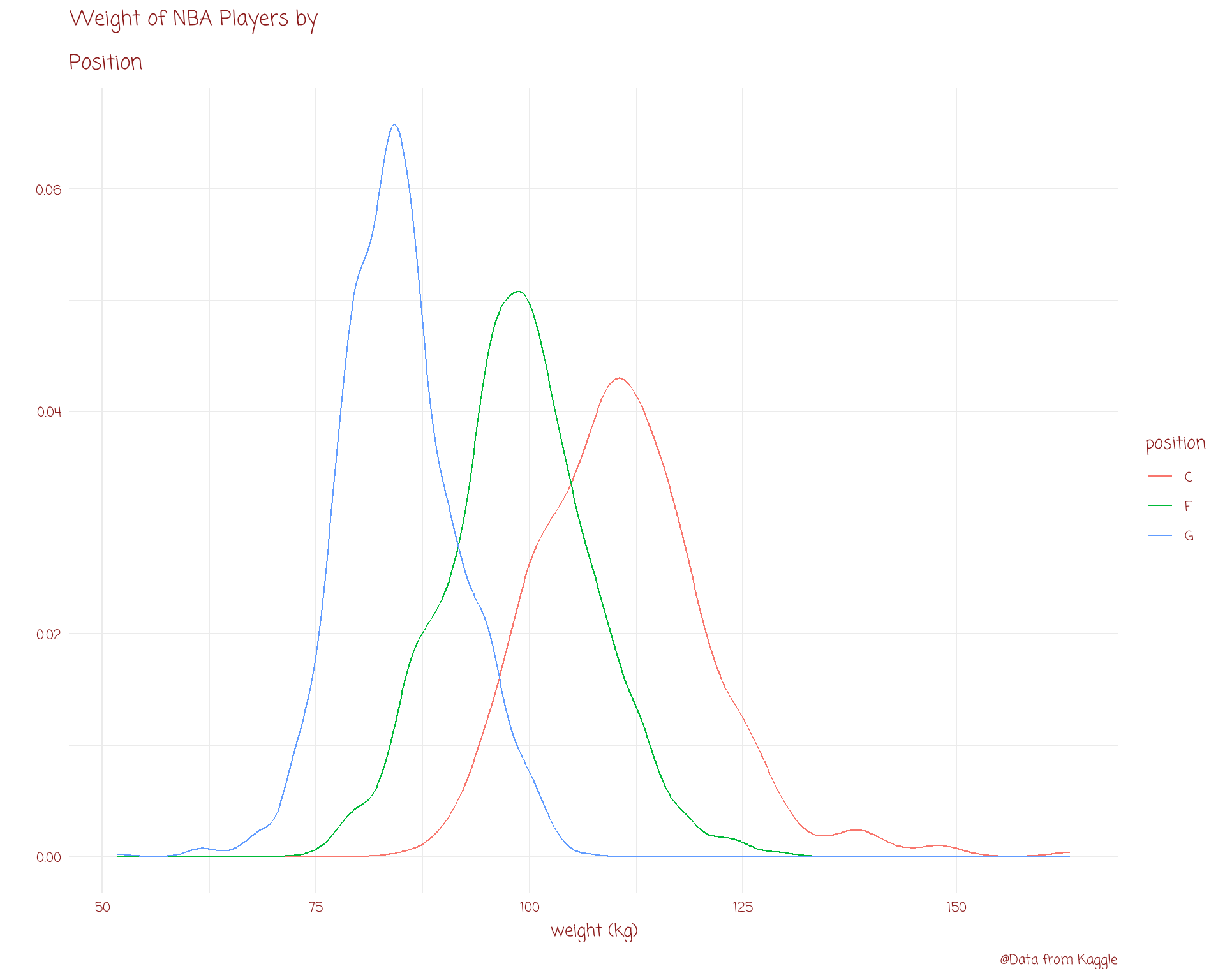
Density Plot
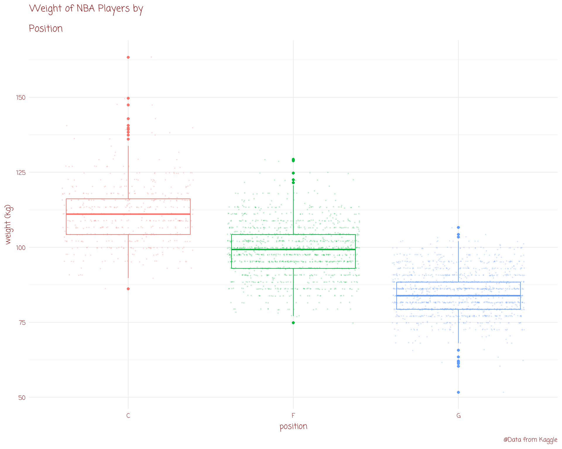
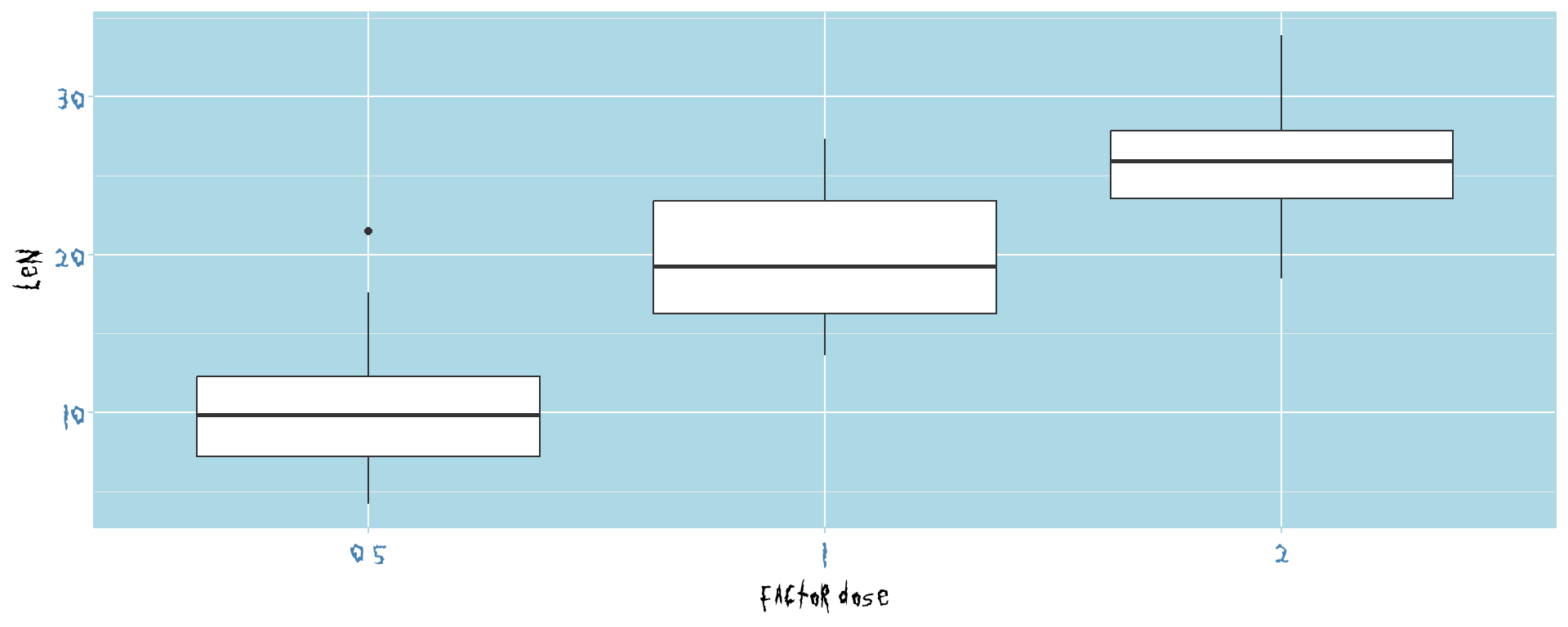
Boxplot

Boxplot
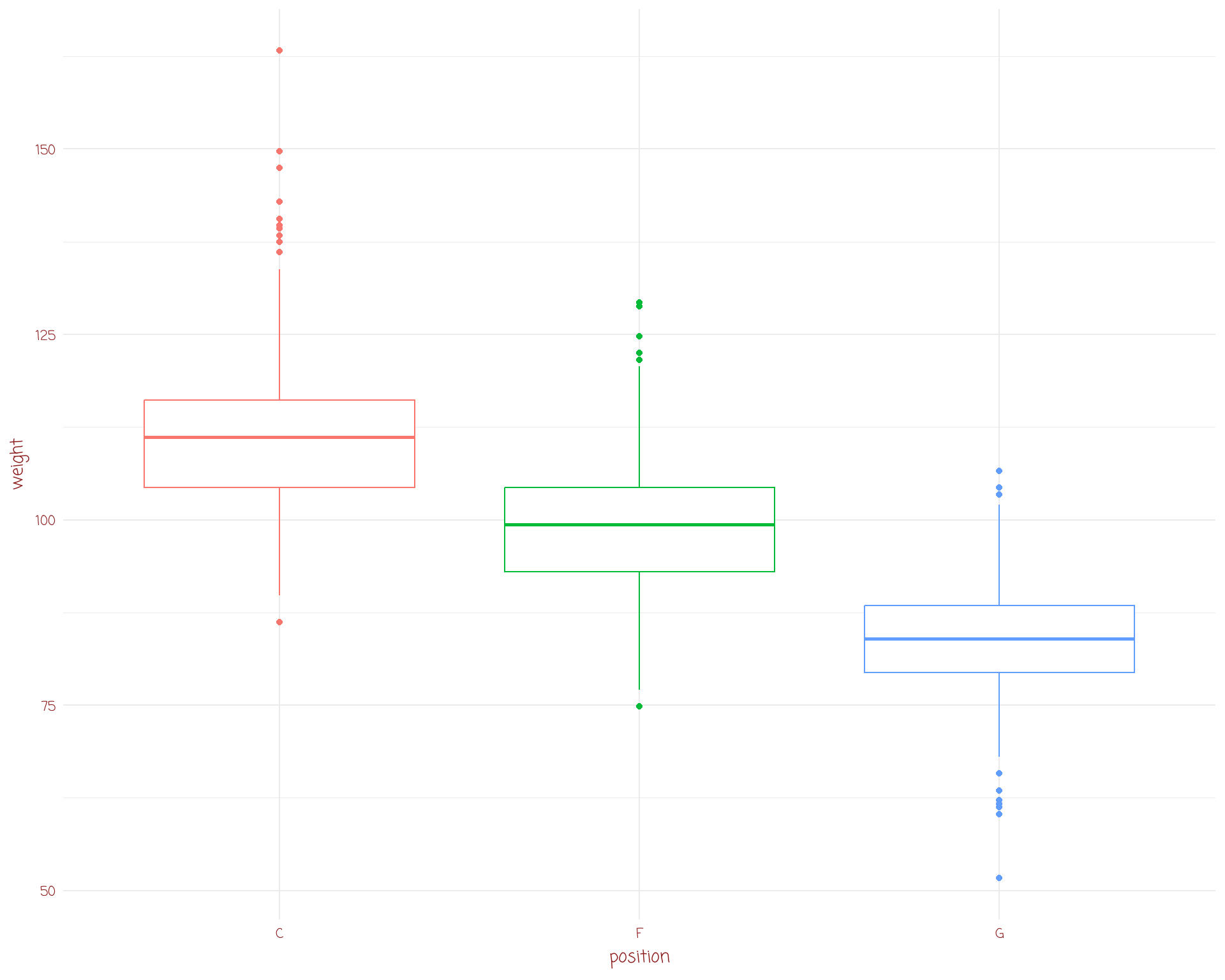
Boxplot
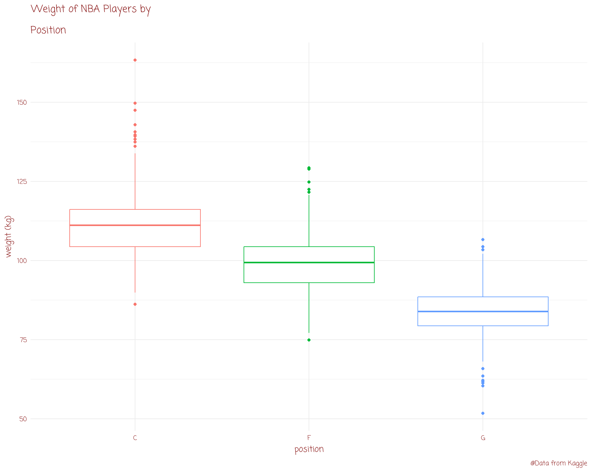
Boxplot
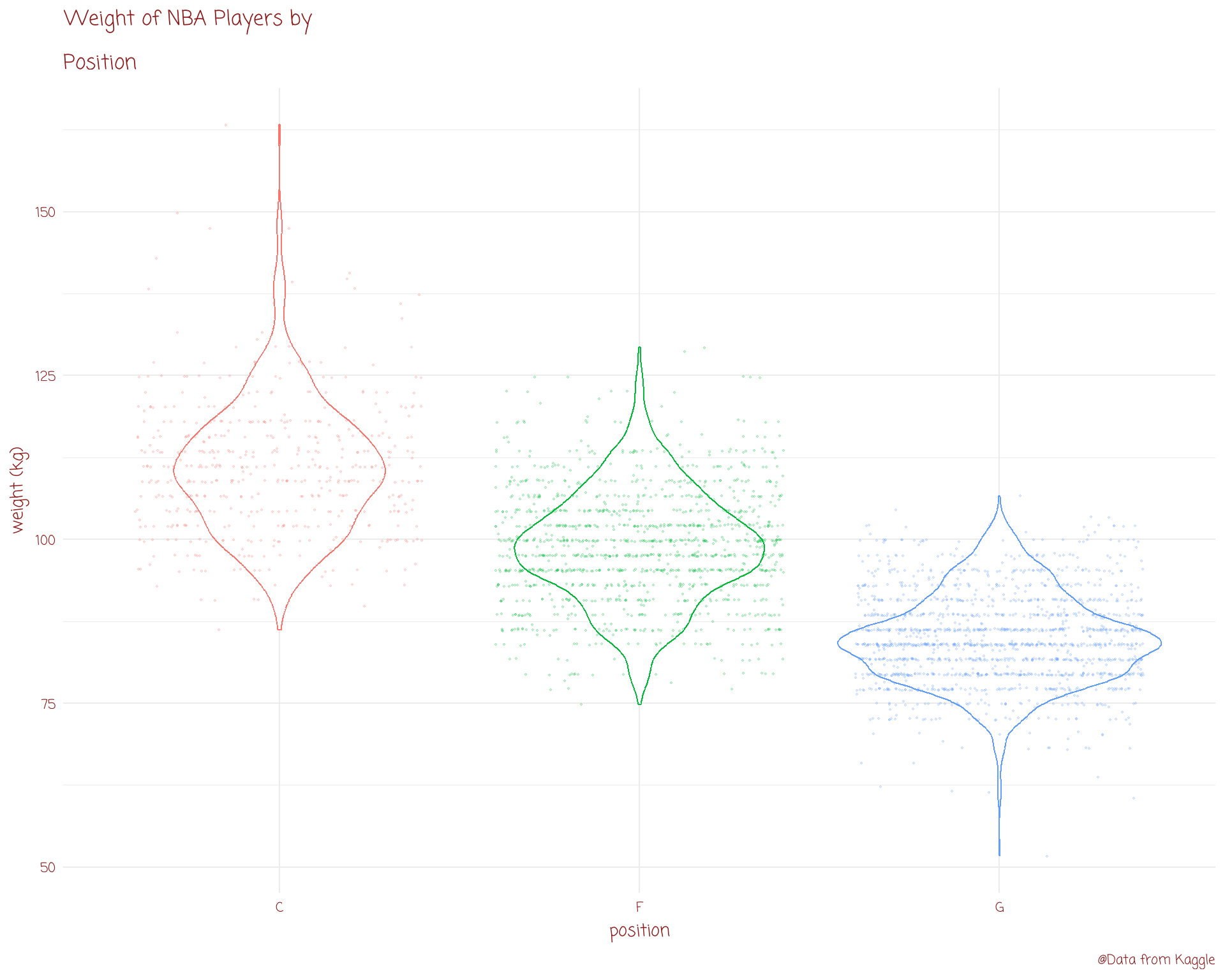
Violin Plot
Violin Plot
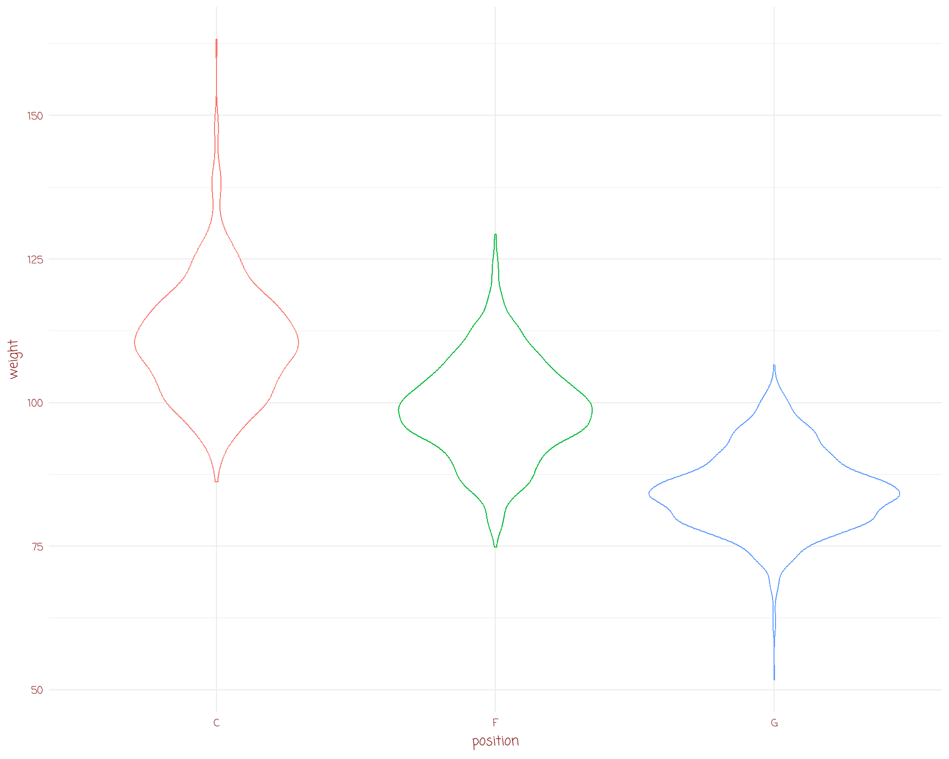
Violin Plot
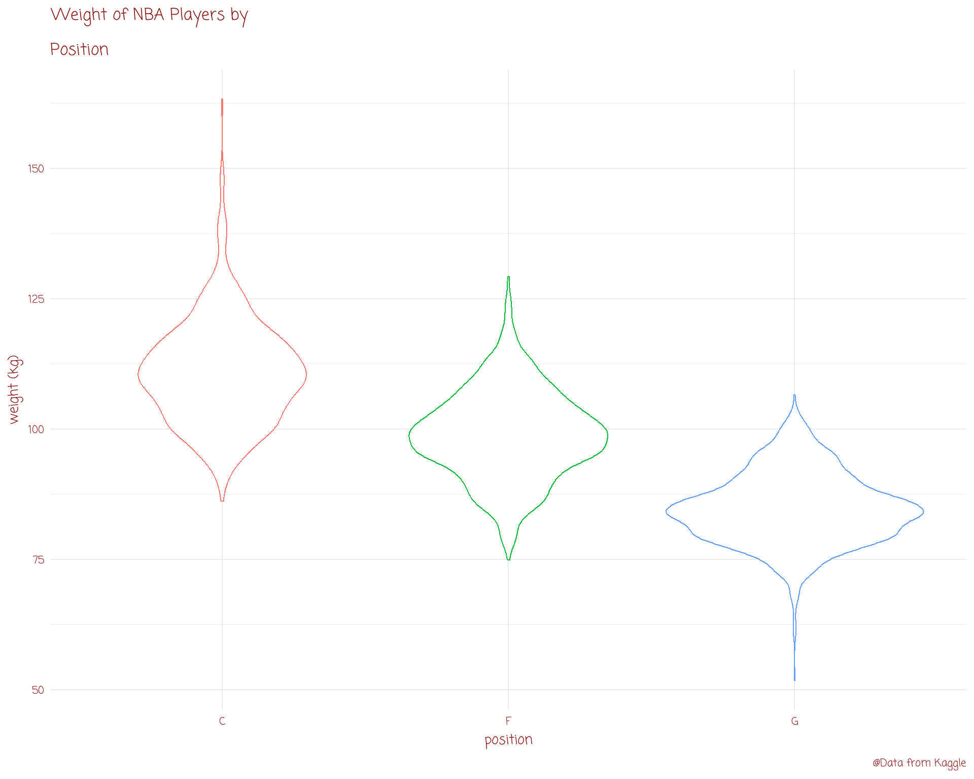
Violin Plot
Ridge Plot
Ridge Plot
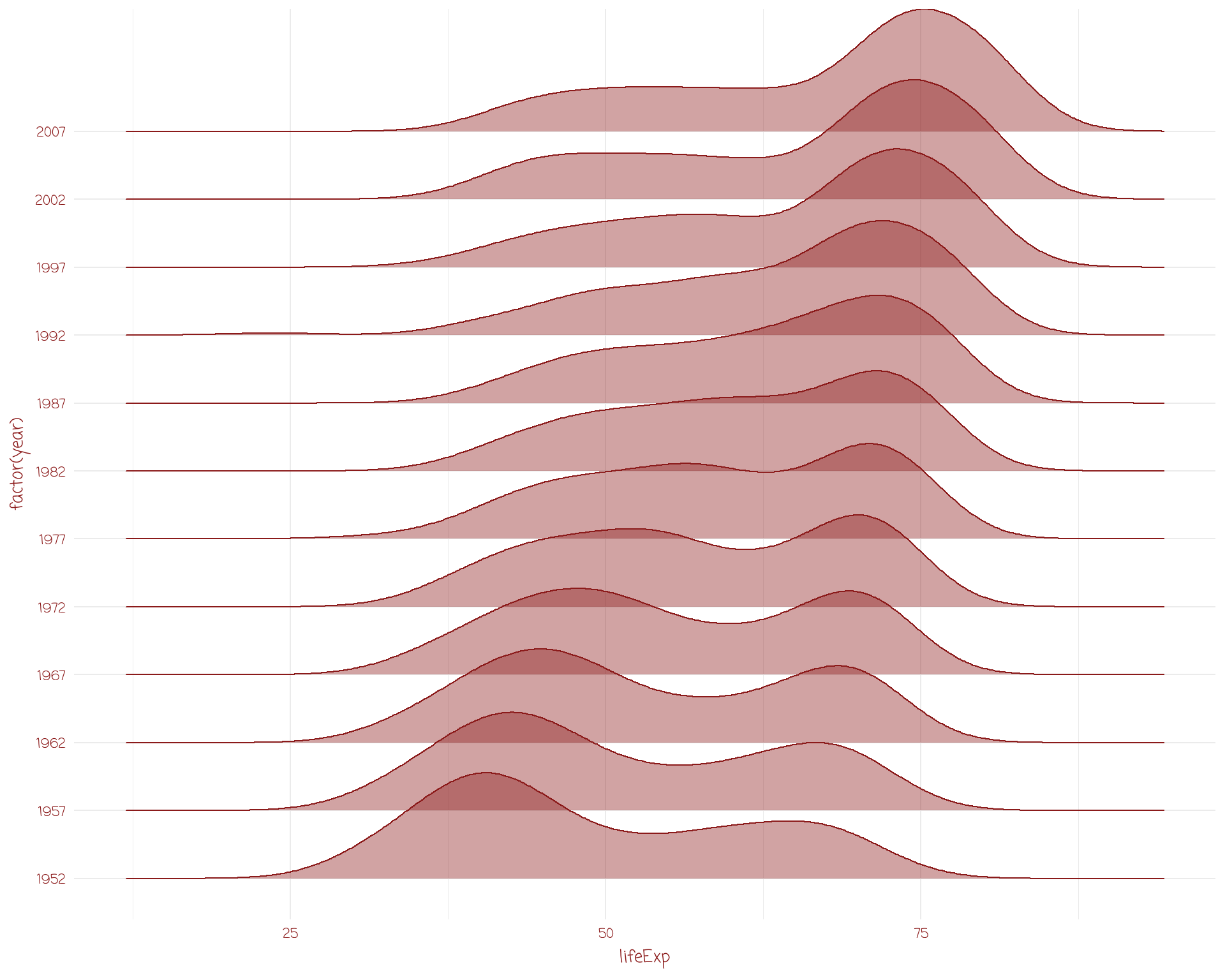
Ridge Plot
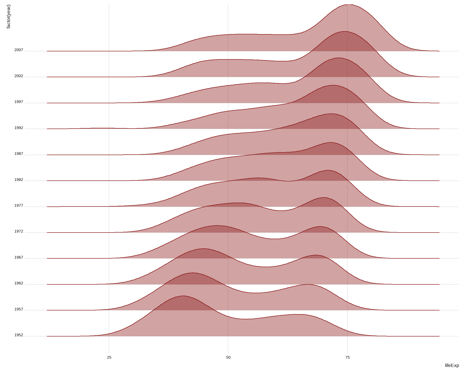
Ridge Plot
Encircle
Encircle
Encircle
Encircle

Encircle
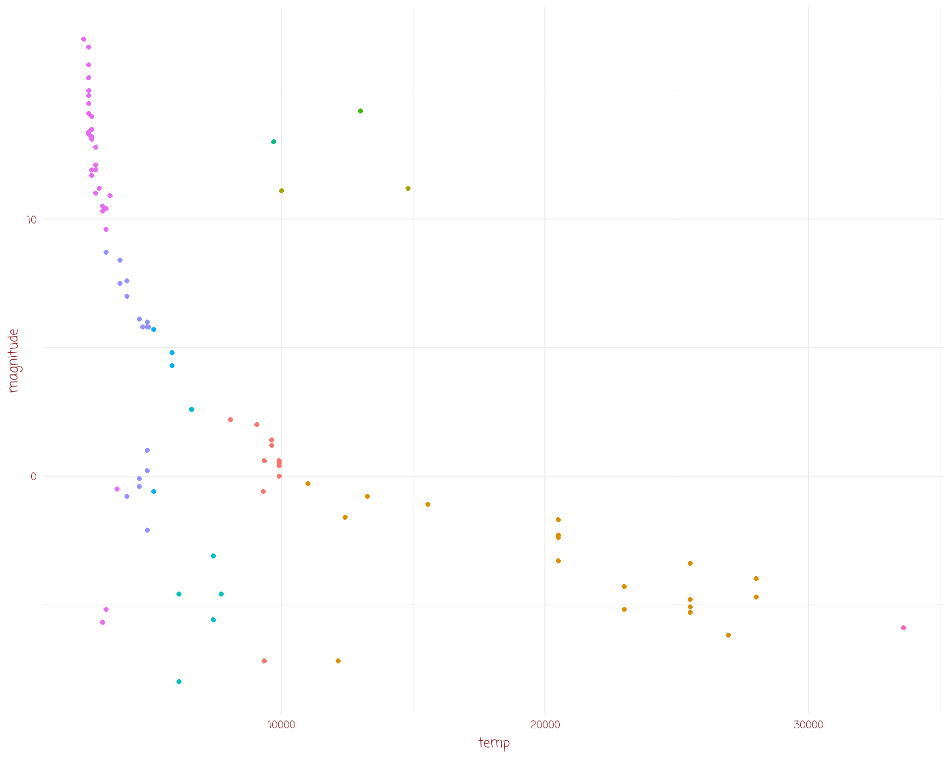
dslabs::stars %>%
  ggplot(aes(temp,
             magnitude,
col = type)) +
geom_point(show.legend = F) +
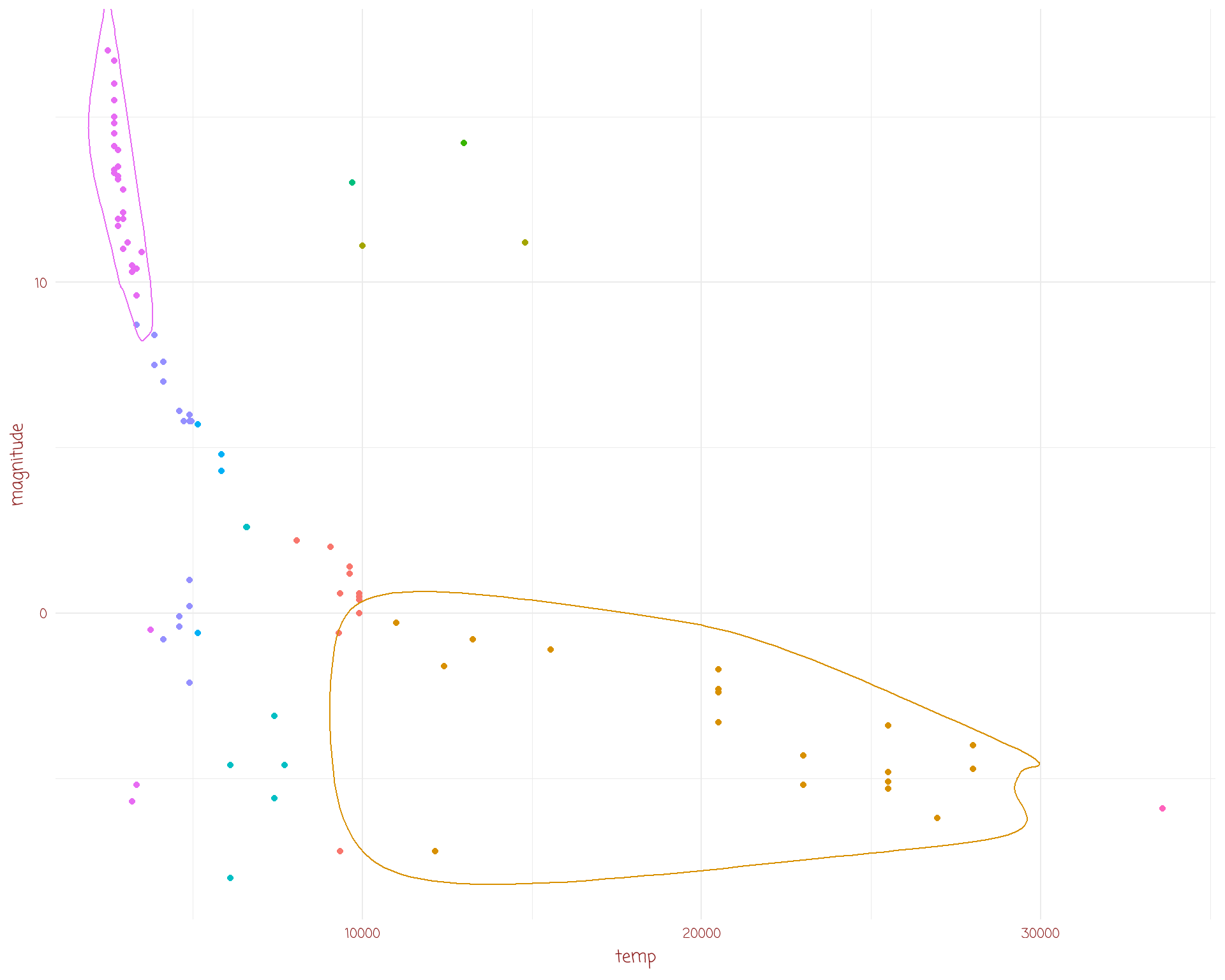
geom_encircle(data = dslabs::stars %>%
dplyr::filter(type == "B" | (type == "M" & magnitude > 9)),
show.legend = F) +
scale_x_log10() +
annotate("text",
x = c(15000, 5000),
y = c(-4, 14),
label = c("Type B Stars", "Faint Type M Stars"),
col = c("blue", "olivedrab3"),
family = "Ink Free",
size = 4,
fontface = 2)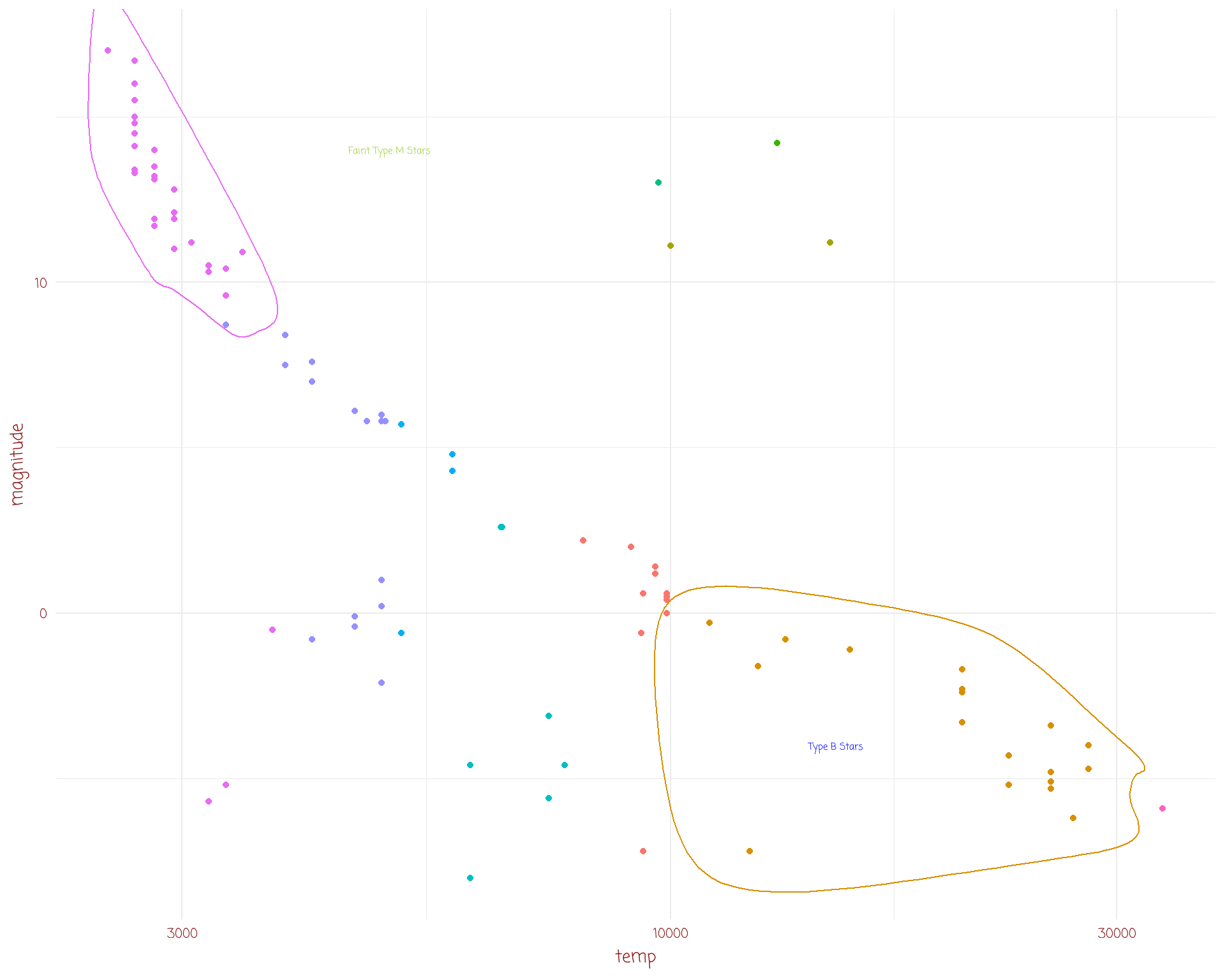
Encircle
dslabs::stars %>%
  ggplot(aes(temp,
             magnitude,
             col = type)) +
geom_point(show.legend = F) +
geom_encircle(data = dslabs::stars %>%
dplyr::filter(type == "B" | (type == "M" & magnitude > 9)),
show.legend = F) +
scale_x_log10() +
annotate("text",
x = c(15000, 5000),
y = c(-4, 14),
label = c("Type B Stars", "Faint Type M Stars"),
col = c("blue", "olivedrab3"),
family = "Ink Free",
size = 4,
fontface = 2) +
scale_color_viridis_d()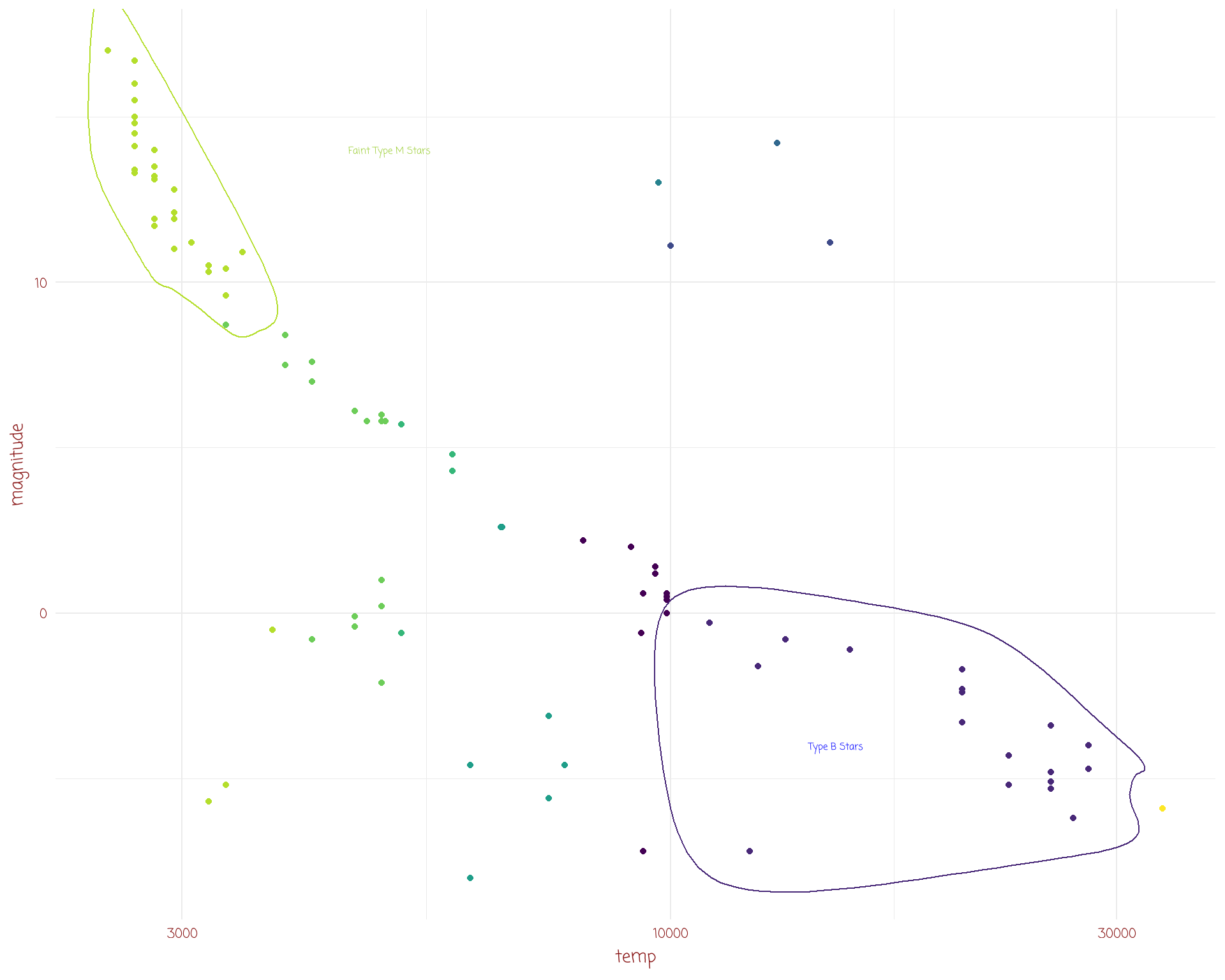
Types of Colour Scales
qualitative
- suite of colours that are easily distinguished
- no heirarchy
- caters for visual impairments

sequential
- band of colours that are increasingly intense
- go from low to high

diverging
- suite of colours that go from minus to plus
- contrasting colours at each end
- something bland and neutral in the middle

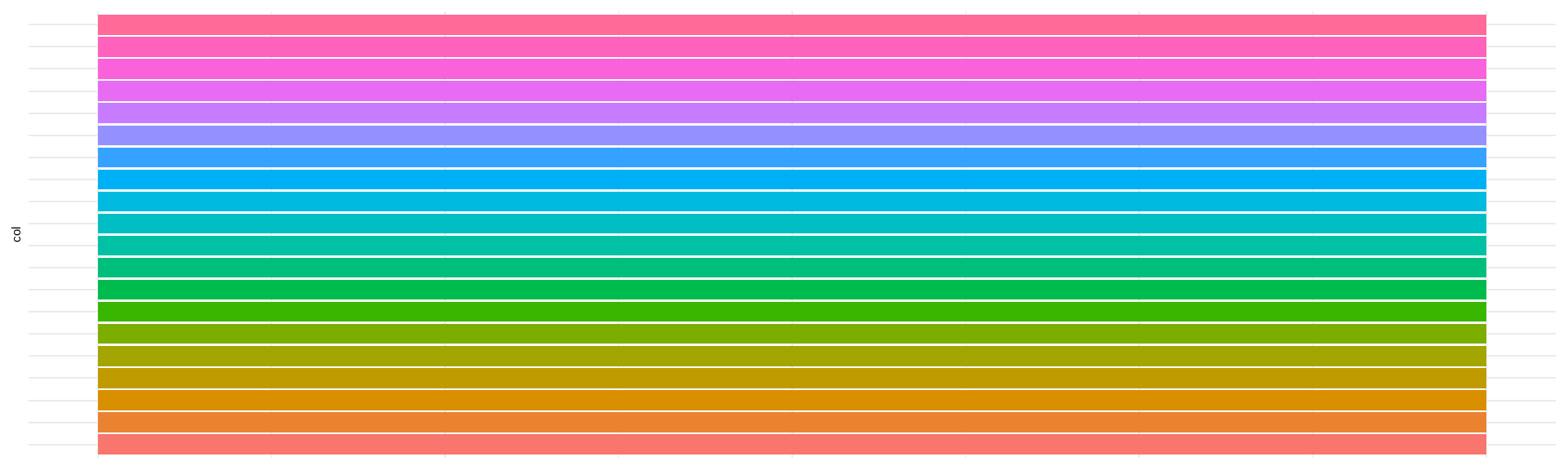
Investigating Colours in R
- the following code shows the first “N” colours in R where N is set to 20 here:
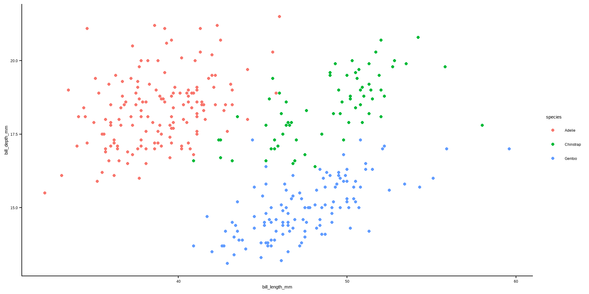
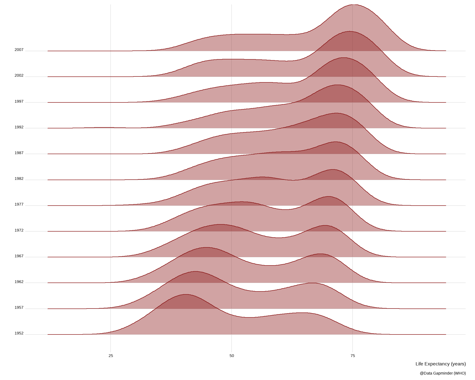
Assignment - Week Five
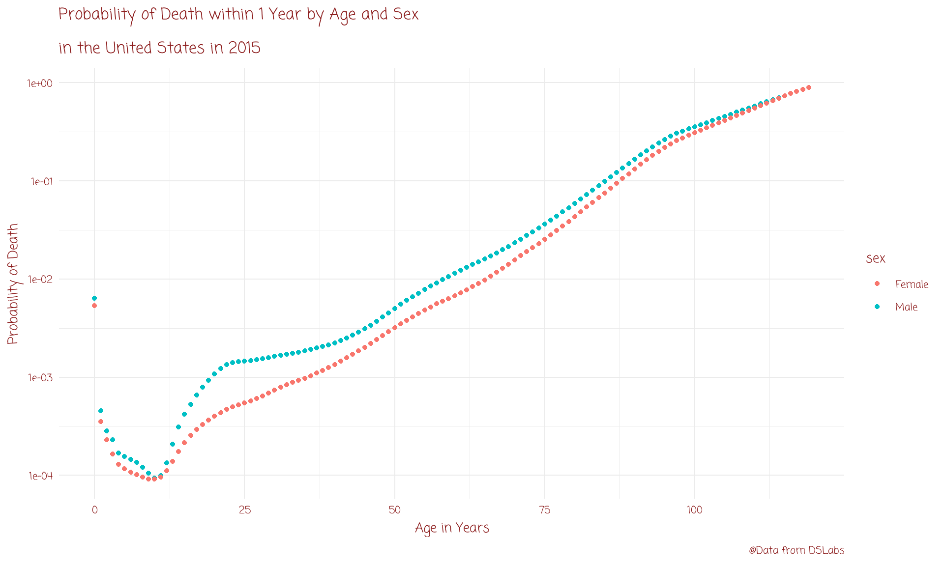
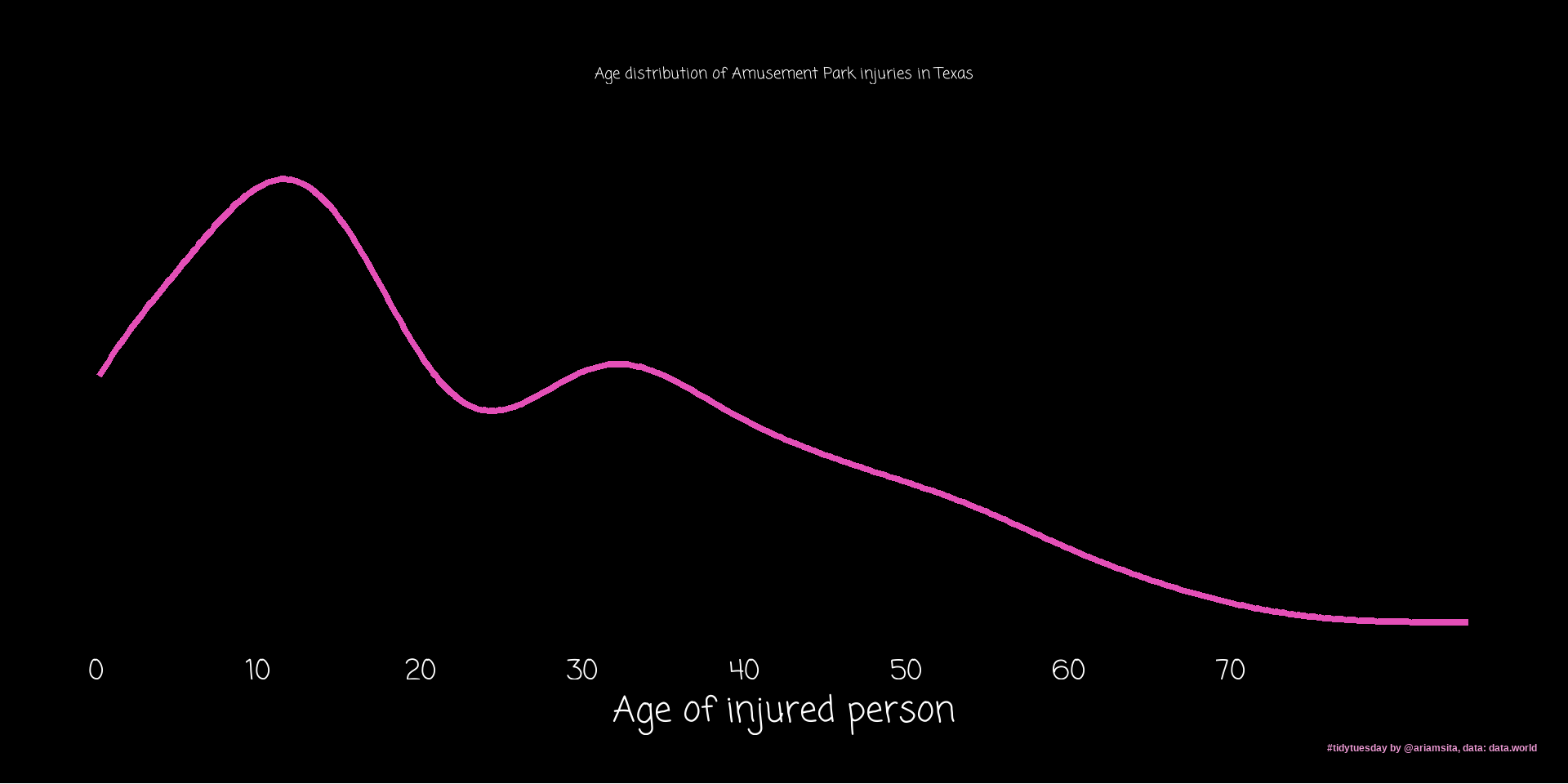
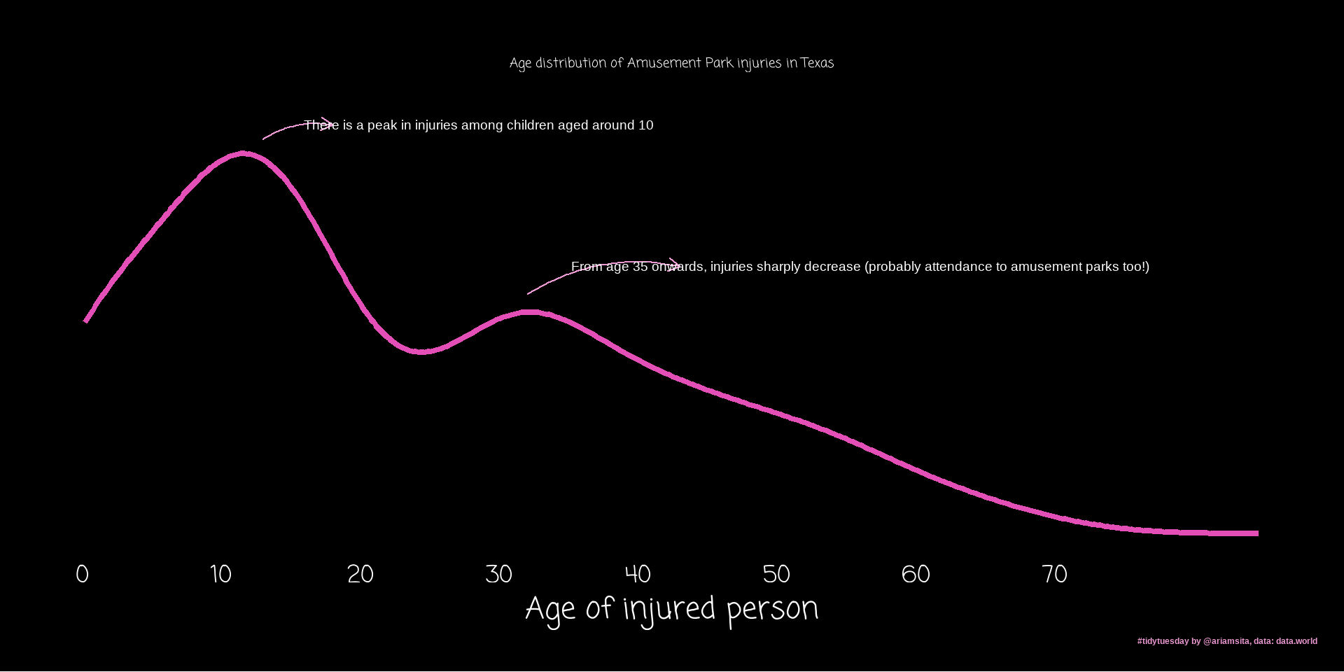
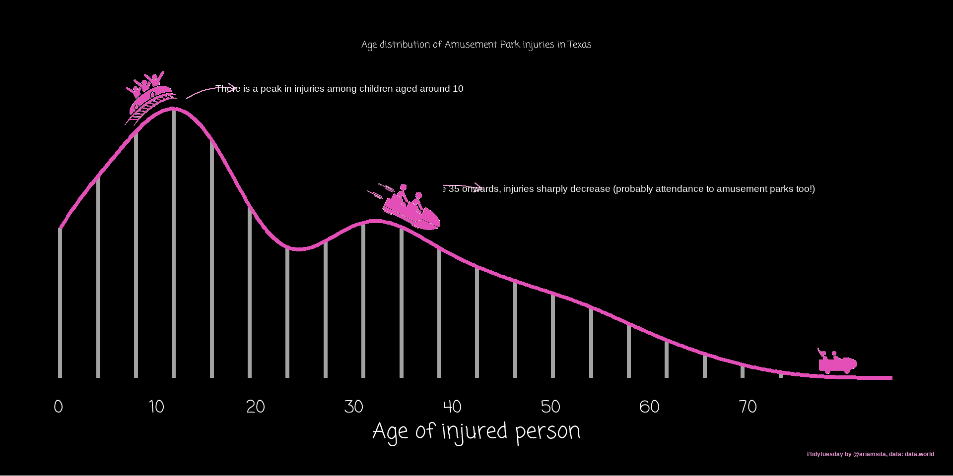
You are tasked with reproducing the following figure: